Gibbs biclustering of microarray data
Gibbs biclustering of microarray data. Yves Moreau & Qizheng Sheng Katholieke Universiteit Leuven ESAT-SCD (SISTA) on leave at Center for Biological Sequence analysis, Danish Technical University. Clustering. Form coherent groups of Genes Patient samples (e.g., tumors)

Gibbs biclustering of microarray data
E N D
Presentation Transcript
Gibbs biclustering of microarray data Yves Moreau & Qizheng Sheng Katholieke Universiteit LeuvenESAT-SCD (SISTA) on leave at Center for Biological Sequence analysis, Danish Technical University
Clustering • Form coherent groups of • Genes • Patient samples (e.g., tumors) • Drug or toxin response • Study these groups to get insight into biological processes • Diagnostic and prognostic classes • Genes in same clusters can have same function or same regulation • Clustering algorithms • Hierarchical clustering • K-means • Self-Organizing Maps • ... CBS Microarray Course
What’s wrong with clustering? • Clustering is a long-solved problem ?!? • Many problems with current clustering algorithms • PCA does not do any form of grouping • Hierarchical clustering does not produce distinct groups • Only a tree; it is then up to the user to pick nodes from the tree • K-means does not tell you how many clusters really are present in the data • ... CBS Microarray Course
A wish list for clustering • We expect a lot from a clustering algorithm • Fast and not memory hungry • Can run easily on a large microarray data set • 10-100.000 genes, >100 experiments • Partitioning of genes into distinct groups and automatically determine the “right” number of groups • Robust • If you remove some genes and some experiments, you want to obtain roughly the same groups • Rejection of outliers (genes that do not clearly belong to any group) • Probabilistic cluster membership • One gene can belong to several clusters • Incorporation of biological knowledge into account • Maybe you want some known genes to cluster together • Meaning of the clusters? • Heterogeneous microarray data sources CBS Microarray Course
Biclustering microarray data CBS Microarray Course
From genome projects to transcriptome projects • Microarray cost per expression measurement • Budgets and expertise • Publicly available microarray data • Need for exchange standards & repositories • Big consortia set up big microarray projects • Genome projects “transcriptome” projects (= compendia) • Change in microarray projects ( sequence analysis) • Analyze public data first to generate an hypothesis • Design and perform your own microarray experiment CBS Microarray Course
Why biclustering? • Data becomes more heterogeneous • Gene clustering • Group genes that behave similarly over all conditions • Gene biclustering • Group genes that behave similarlyover a subset of conditions • “Feature selection” • More suitable for heterogeneous compendium CBS Microarray Course
Genetics Sequence analysis Linkage analysis Phylogeny Modeling protein families Gene prediction Regulatory sequence analysis Graphicalmodels Biostatistics Expression analysis Bayesian stats Clustering Decision support Clustering Genetic network inference Probabilistic graphical models CBS Microarray Course
Discretized microarray data set Discretizing microarray data Microarray data is continuous Discretize by equal frequency High Medium Low Distribution of expression values for a given gene Bicluster genes conditions CBS Microarray Course
Bicluster CBS Microarray Course
1 0 Pattern Background Likelihood CBS Microarray Course
1 0 Likelihood .9.9.9.9.9 .9.05.9.9.9 .9.9.9.9.9 .05.9.9.9.9 .9.9.9.9.05 CBS Microarray Course
1 0 Likelihood Get the right genes .9.05.05.05.9 .05.9.9.05.05 .05.05.05.05.05 .05.05.9.9.05 CBS Microarray Course
1 Likelihood 0 Get the right conditions .9.9.05.05.9 .9.05.05.9.9 .9.9 .05 .05.9 .05.9.05 .05.9 .9.9 .05 .05.05 CBS Microarray Course
1 Likelihood 0 Get the right frequency pattern .6.6.2.2.6 .6.2.2.2.6 .6.6.2.2.6 .2.6.2.2.6 .2.6.2.2.2 CBS Microarray Course
Optimizing the bicluster • Find the right bicluster • Genes • Conditions • Pattern • For a given choice of genes and conditions, the “best” pattern is given by the frequencies found in the extracted pattern • No more need to optimize over the pattern • Maximum likelihood: find genes and conditions that maximize • Gibbs sampling: find genes and conditions that optimize CBS Microarray Course
Gibbs sampling CBS Microarray Course
Markov Chain Monte-Carlo • Markov chain with transition matrix T A C G T A0.0643 0.8268 0.0659 0.0430 C 0.0598 0.0484 0.8515 0.0403 G 0.1602 0.3407 0.1736 0.3255 T 0.1507 0.1608 0.3654 0.3231 X=A X=T X=C X=G CBS Microarray Course
Markov Chain Monte-Carlo • Markov chains can sample from complex distributions ACGCGGTGTGCGTTTGACGA ACGGTTACGCGACGTTTGGT ACGTGCGGTGTACGTGTACG ACGGAGTTTGCGGGACGCGT ACGCGCGTGACGTACGCGTG AGACGCGTGCGCGCGGACGC ACGGGCGTGCGCGCGTCGCG AACGCGTTTGTGTTCGGTGC ACCGCGTTTGACGTCGGTTC ACGTGACGCGTAGTTCGACG ACGTGACACGGACGTACGCG ACCGTACTCGCGTTGACACG ATACGGCGCGGCGGGCGCGG ACGTACGCGTACACGCGGGA ACGCGCGTGTTTACGACGTG ACGTCGCACGCGTCGGTGTG ACGGCGGTCGGTACACGTCG ACGTTGCGACGTGCGTGCTG ACGGAACGACGACGCGACGC ACGGCGTGTTCGCGGTGCGG % A C G Position T CBS Microarray Course
Gibbs sampling • Markov chain for Gibbs sampling CBS Microarray Course
Gibbs sampling • True target distribution (2D normal N(m,s)) CBS Microarray Course
Gibbs sampling • First 20 Gibbs sampling iterates (conditionals are 1D normals) CBS Microarray Course
Gibbs sampling • Burn-in samples (1000 samples) CBS Microarray Course
Gibbs sampling • Samples after Markov chain convergence (samples 1000-2000) CBS Microarray Course
Data augmentation Gibbs sampling • Introducing unobserved variables often simplifies the expression of the likelihood • A Gibbs sampler can then be set up • Samples from the Gibbs sampler can be used to estimate parameters CBS Microarray Course
Pros and cons • Gibbs sampling • Explore the space of configuration of a probabilistic model of the data according to the probability of each configuration • Based on incrementaly perturbing the configuration one variable at a time, preferably choosing more likely configurations • Pros • Clear probabilistic interpretation • Bayesian framework • “Global optimization” • Cons • Mathematical details not easy to work out • Relatively slow CBS Microarray Course
Gibbs biclustering CBS Microarray Course
Gibbs sampling Current configuration Next gene configuration CBS Microarray Course
Updated gene configuration Next complete configuration iterate many times CBS Microarray Course
Gibbs biclustering CBS Microarray Course
Simulated data CBS Microarray Course
Remarks • Gibbs biclustering allows noisy patterns • Optimized configuration is obtained by averaging successive iterated configurations • Biclustering is oriented • Find subset of samples for which a subset of genes is consistenly expressed across genes • Find subset of genes that are consistently expressed across a subset of samples • Searching for multiple patterns • For gene biclustering, remove the data of the genes from the current bicluster • Search for a new pattern • Stop if only empty pattern repeatedly found CBS Microarray Course
Multiple biclusters CBS Microarray Course
Leukemia fingerprints CBS Microarray Course
Mixed-Lineage Leukemia • Armstrong et al., Nature Genetics, 2002 • Mixed-Lineage Leukemia (MLL) is a subtype of ALL • Caused by chromosomal rearrangement in MLL gene • Poorer prognosis than ALL • Microarray analysis shows that MLL is distinct from ALL • FLT3 tyrosine kinase distinguishes most strongly between MLL, ALL, and AML • Candidate drug target CBS Microarray Course
PCA Features CBS Microarray Course
Biclustering leukemia data • Bicluster patients • Find patients for which a subset of genes has a consistent expression profile across this group of patients • Discovery set • 21 ALL, 17 MLL, 25 AML • Validation set • 3 ALL, 3 MLL, 3 AML CBS Microarray Course
Discovering ALL • Bicluster 1: 18 out of 21 ALL patients CBS Microarray Course
Discovering MLL • Bicluster 2: 14 out of 17 MLL patients CBS Microarray Course
Discovering AML • Bicluster 3: 19 out of 25 AML patients CBS Microarray Course
Rescoring ALL CBS Microarray Course
Rescoring MLL CBS Microarray Course
Rescoring AML CBS Microarray Course
K.U.Leuven ESAT-SCD-Bioi Qizheng Sheng