Understanding Sequence Alignment via HMM Model Structures
200 likes | 284 Vues
Learn about Markov chain limitations and Hidden Markov Model structures for sequence alignment, including silent states, high-order chains, and inhomogeneous chains. Explore genetic code, emission probabilities, and scoring functions for HMMs in alignment.

Understanding Sequence Alignment via HMM Model Structures
E N D
Presentation Transcript
Sequence Alignment via HMM Background Readings: chapters 3.4, 3.5, 4, in the Durbin et al. .
A1 A2 A3 A4 HMM model structure:1. Duration Modeling Markov chains are rather limited in describing sequences of symbols with non-random structures. For instance, Markov chain forces the distribution of segments in which some state is repeated for k times to be (1-p)pk-1, for some p. Several ways enable modeling of other distributions. One is assigning k >1 states to represent the same “real” state. This may guarantee k repetitions with any desired probability.
HMM model structure:2. Silent states • States which do not emit symbols (as we saw in the abo locus). • Can be used to model duration distributions. • Also used to allow arbitrary jumps (may be used to model deletions) • Need to generalize the Forward and Backward algorithms for arbitrary acyclic digraphs to count for the silent states (see next): Silent states: Regular states:
Eg, the forwards algorithm should look: z Silent states Directed cycles of silence (or other) states complicate things, and should be avoided. Regular states v x symbols
HMM model structure:3. High Order Markov Chains Markov chains in which the transition probabilities depends on the last n states: P(xi|xi-1,...,x1) = P(xi|xi-1,...,xi-n) Can be represented by a standard Markov chain with more states: AA AB BB BA
HMM model structure:4. Inhomogenous Markov Chains • An important task in analyzing DNA sequences is recognizing the genes which code for proteins. • A triplet of 3 nucleotides – called codon - codes for amino acids (see next slide). • It is known that in parts of DNA which code for genes, the three codons positions has different statistics. • Thus a Markov chain model for DNA should represent not only the Nucleotide (A, C, G or T), but also its position – the same nucleotide in different position will have different transition probabilities. This seems to work better in some cases (see eg Durbin et al, p. 76)
Genetic Code There are 20 amino acids from which proteins are build.
Sequence Comparison using HMM HMM for sequence alignment, which incorporates affine gap scores. “Hidden” States • Match • Insertion in x • insertion in y. Symbols emitted • Match: {(a,b)| a,b in∑ } • Insertion in x: {(a,-)| a in ∑ }. • Insertion in y: {(-,a)| a in ∑ }.
M X Y 1-2δ δ δ M 1- ε ε X 1- ε ε Y The Transition Probabilities • Emission Probabilities • Match: (a,b) with pab – only from M states • Insertion in x: (a,-) with qa – only from X state • Insertion in y: (-,a).with qa - only from Y state. Transitions probabilities (note the forbidden ones). δ= probability for 1st gap ε = probability for tailing gap.
The Transition Probabilities Each aligned pair is generated by the above HMM with certain probability. Note that the hidden states can be reconstructed from the alignment. However, for each pair of sequences x (of length m)and y (of length n), there are many alignments of x and y, each corresponds to a different state-path (the length of the paths are between max{m,n} and m+n). Our task is to score alignments by using this model. The score should reflect the probability of the alignment.
Most probable alignment Let vM(i,j) be the probability of the most probable alignment of x(1..i) and y(1..j), which ends with a match. Then using a recursive argument, we get:
Most probable alignment Similarly, vX(i,j) and vY(i,j), the probabilities of the most probable alignment of x(1..i) and y(1..j), which ends with an insertion to x or y:
Adding termination probabilities We may want a model which defines a probability distribution over all possible sequences. For this, an END state is added, with transition probability τ from any other state to END. This assume expected sequence length of 1/ τ.
Full probability of x and y Rather then computing the probability of the most probable alignment, we look for the total probability that x and y are related by our model. Let fM(i,j) be the sum of the probabilities of all alignments of x(1..i) and y(1..j), which end with a match. Similarly, fX(i,j) and fY(i,j) are the sum of these alignments which end with insertion to x (y resp.). A “forward” type algorithm for computing these functions. Initialization: fM(0,0)=1, fX(0,0)= fY(0,0)=0 (we start from M, but we could select other initial state).
Full probability of x and y (cont.) The total probability of all alignments is: P(x,y|model)= fM[m,n] + fX[m,n] + fY[m,n]
The log-odds scoring function • We wish to know if the alignment score is above or below the score of random alignment. • Recall: The log-odds ratio s(a,b) = log (pab /qaqb). • log (pab/qaqb)>0 iff the probability that a and b are related by our model is larger than the probability that they are picked at random. • To adapt this for the HMM model, we need to model random sequence by HMM, with end state.
The log-odds scoring function The transition probabilities for the random model: (x is the start state) The emission probability for a is qa. Thus the probability of of x (of length n) and y (of length m) being random is:
Markov Chains for “Random” and “Model” “Random” “Model”
The log-odds scoring function The resulted scoring function s in the HMM model: d and e are the penalties for a first gap and a tailing gap, resp, which are subtracted from the score. The algorithm corrects for extra prepayment, as follows:
Log-odds alignment algorithm Initialization: VM(0,0)=logτ - 2logη. Termination: V = max{ VM(m,n), VX(m,n)+c, VY(m,n)+c} Where c= log (1-2δ-τ) – log(1-ε-τ)