Deterministic Chaos
Deterministic Chaos. caoz. PHYS 306/638 University of Delaware. Chaos vs. Randomness. Do not confuse chaotic with random: Random: irreproducible and unpredictable Chaotic:


Deterministic Chaos
E N D
Presentation Transcript
Deterministic Chaos caoz PHYS 306/638 University of Delaware
Chaos vs. Randomness • Do not confuse chaotic with random: Random: • irreproducible and unpredictable Chaotic: • deterministic - same initial conditions lead to same final state… but the final state is very different for small changes to initial conditions • difficult or impossible to make long-term predictions
Suppose the Universe is made of particles of matter interacting according to Newton laws→ this is just a dynamical system governed by a (very large though) set of differential equations • Given the starting positions and velocities of all particles, there is a unique outcome → P. Laplace’sClockwork Universe (XVIII Century)! Clockwork (Newton) vs. Chaotic (Poincaré) Universe
Chaos in the Brave New World of Computers • Poincaré created an original method to understand such systems, and discovered a very complicated dynamics,but: "It is so complicated that I cannot even draw the figure."
An Example… A Pendulum • starting at 1, 1.001, and 1.000001 rad:
Changing the Driving Force • f = 1, 1.07, 1.15, 1.35, 1.45
Chaos in Physics • Chaos is seen in many physical systems: • Fluid dynamics (weather patterns), • some chemical reactions, • Lasers, • Particle accelerators, … • Conditions necessary for chaos: • system has 3 independent dynamical variables • the equations of motion are non-linear
Dynamical Systems • A dynamical system is defined as a deterministic mathematical prescription for evolving the state of a system forward in time • Example: A system of N first-order, autonomous ODE
Damped Driven Pendulum: Part I • This system demonstrates features of chaotic motion: • Convert equation to a dimensionless form: q q 2 d d + + q = w + f ml c mg sin A cos( t ) D 2 dt dt w q d d + + q = w q sin f cos( t ) 0 D dt dt
Damped Driven Pendulum: Part II • 3 dynamic variables:, , t • the non-linear term: sin • this system is chaotic only for certain values of q, f0 , and wD • In these examples: • wD = 2/3, q = 1/2, and f0 near 1
Damped Driven Pendulum: Part III • to watch the onset of chaos (as f0 is increased) we look at the motion of the system in phase space, once transients die away • Pay close attention to the period doubling that precedes the onset of chaos...
= f 1 . 07 0 = f 1 . 15 0
f0 = 1.35 f0 = 1.45 f0 = 1.47 f0 = 1.48 f0 = 1.49 f0 = 1.50
Forget About Solving Equations! New Language for Chaos: • Attractors (Dissipative Chaos) • KAM torus (Hamiltonian Chaos) • Poincare sections • Lyapunov exponents and Kolmogorov entropy • Fourier spectrum and autocorrelation functions
Poincaré Section: Pendulum • The Poincaré section is a slice of the 3D phase space at a fixed value of: Dt mod 2 • This is analogous to viewing the phase space development with a strobe light in phase with the driving force. Periodic motion results in a single point, period doubling results in two points...
Poincaré Movie • To visualize the 3D surface that the chaotic pendulum follows, a movie can be made in which each frame consists of a Poincaré section at a different phase... • Poincare Map: Continuous time evolution is replace by a discrete map
f0 = 1.07 f0 = 1.48 f0 = 1.50 f0 = 1.15 q = 0.25
Attractors • The surfaces in phase space along which the pendulum follows (after transient motion decays) are called attractors • Examples: • for a damped undriven pendulum, attractor is just a point at =0. (0D in 2D phase space) • for an undamped pendulum, attractor is a curve (1D attractor)
Strange Attractors • Chaotic attractors of dissipative systems (strange attractors) are fractals Our Pendulum: 2 < dim < 3 • The fine structure is quite complex and similar to the gross structure: self-similarity. non-integer dimension
N N 1 L 1 L 2 L/2 4 L/2 4 L/4 16 L/4 8 L/8 22n L/2n 2n L/2n What is Dimension? • Capacity dimension of a line and square: = e d d N ( e ) L ( 1 / ) = e e d lim log N ( ) / log( 1 / ) c e ® 0
2 1/3 4 1/9 8 1/27 = n n d lim log 2 / log 3 c ® ¥ n = < d log 2 / log 3 1 c Non-Trivial Example: Cantor Set • The Cantor set is produced as follows: N 1 1
Lyapunov Exponents: Part I • The fractional dimension of a chaotic attractor is a result of the extreme sensitivity to initial conditions. • Lyapunov exponents are a measure of the average rate of divergence of neighbouring trajectories on an attractor.
e1t e2t Lyapunov Exponents: Part II • Consider a small sphere in phase space… after a short time the sphere will evolve into an ellipsoid:
Lyapunov Exponents: Part III • The average rate of expansion along the principle axes are the Lyapunov exponents • Chaos implies that at least one is > 0 • For the pendulum: i = -q (damp coeff.) • no contraction or expansion along t direction so that exponent is zero • can be shown that the dimension of the attractor is: d = 2 - 1 / 2
Dissipative vs Hamiltonian Chaos • Attractor:An attractor is a set of states (points in the phase space), invariant under the dynamics, towards which neighboring states in a given basin of attraction asymptotically approach in the course of dynamic evolution. An attractor is defined as the smallest unit which cannot be itself decomposed into two or more attractors with distinct basins of attraction. This restriction is necessary since a dynamical system may have multiple attractors, each with its own basin of attraction. • Conservative systems do not have attractors, since the motion is periodic. For dissipative dynamical systems, however, volumes shrink exponentially so attractors have 0 volume in n-dimensional phase space. • Strange Attractors:Bounded regions of phase space (corresponding to positive Lyapunov characteristic exponents) having zero measure in the embedding phase space and a fractal dimension. Trajectories within a strange attractor appear to skip around randomly
Dissipative vs Conservative Chaos: Lyapunov Exponent Properties • For Hamiltonian systems, the Lyapunov exponents exist in additive inverse pairs, while one of them is always 0. • In dissipative systems in an arbitrary n-dimensional phase space, there must always be one Lyapunov exponent equal to 0, since a perturbation along the path results in no divergence.
= m - x x ( 1 x ) - - 1 1 n n n Logistic Map: Part I • The logistic map describes a simpler system that exhibits similar chaotic behavior • Can be used to model population growth: • For some values of , x tends to a fixed point, for other values, x oscillates between two points (period doubling) and for other values, x becomes chaotic….
= m - x x ( 1 x ) - - 1 1 n n n Logistic Map: Part II • To demonstrate… x n x n - 1
Bifurcation Diagrams: Part I • Bifurcation: a change in the number of solutions to a differential equation when a parameter is varied • To observe bifurcatons, plot long term values of , at a fixed value of Dt mod 2 as a function of the force term f0
Bifurcation Diagrams: Part II • If periodic single value • Periodic with two solutions (left or right moving) 2 values • Period doubling double the number • The onset of chaos is often seen as a result of successive period doublings...
Feigenbaum Number • The ratio of spacings between consecutive values of at the bifurcations approaches a universal constant, the Feigenbaum number. • This is universal to all differential equations (within certain limits) and applies to the pendulum. By using the first few bifurcation points, one can predict the onset of chaos. m - m = d = - k k 1 lim 4 . 669201 ... m - m ® ¥ k + k 1 k
Deterministic Chaos in PHYS 306/638 • Aperiodic motion confined to strange attractors in the phase space • Points in Poincare section densely fill some region • Autocorrelation function drops to zero, while power spectrum goes into a continuum