Chaos
Chaos Chow Yuen Shan Chu Wai Siu Outline Introduction Brief history of the discovery of chaos Working definition of chaos Chaos in simple deterministic systems Logistic map Higher dimensional models Examples outside Physics Implications History 1890s Poincaré : three – body problem


Chaos
E N D
Presentation Transcript
Chaos Chow Yuen Shan Chu Wai Siu
Outline Introduction Brief history of the discovery of chaos Working definition of chaos Chaos in simple deterministic systems Logistic map Higher dimensional models Examples outside Physics Implications
History 1890s Poincaré: three – body problem 1930s Cartwrightand Littlewood: modeling radio and radar 1940s Kolmogorov: turbulence and astronomical problems 1960s Age of Computer Lorenz: computer weather simulation in meteorology using the rounded off data generated a completely different prediction!
History 1960s Mandelbrot: Recurring patterns at every scale (Self – similarity), “measuring the coast of Britain (Fractional dimensions) 1970s Robert May: Logistic map in biology Simplest deterministic model showing chaotic behavior Mandelbrot Set Graph from http://en.wikipedia.org/wiki/Mandelbrot_set
What is Chaos? Working definition of Chaos: The underlying dynamics is deterministic Sensitive to initial conditions Some global characteristicsdoes not depend on initial conditions (e.g. Lyapunov exponent) (From Hao Bai-Lin, Chaos II, World Scientific 1990)
The logistic map The simplest example of a nonlinear dynamical system is the one dimensional logistic map The dynamical system is deterministicand its dynamics are determined by a single control parameter aandinitial condition x0.
Iterations of the logistic map Graph from Glass Mackey “From Clocks to Chaos”Pages 30-31 Iterated solutions of the logistic function with different control parameters a (a=2.5, period 1 orbit; a=3.25, period 2 orbit; a=3.5, period 4 orbit; a=4, chaos)
Graphical Iterations Graph from http://en.wikipedia.org/wiki/Logistic_map here r=a
Graphical Iterations Graphical iteration of the logistic function with different control parameters a (a=2.5, period 1 orbit; a=3.25, period 2 orbit; a=3.5, period 4 orbit; a=4, chaos) Graph from Glass Mackey “From Clocks to Chaos” Pages 28-29
Fixed points and their stability Fixed points: For a stable fixed point, the iterated values converges to x* independent of the initial value.
Stability of fixed point Consider
Stability of Fixed Points • Super-stable fixed point, which converges very fast • To test the stability of the 2 fixed points:
Multiple Fixed Points It is possible that the trajectory of iteration has more than one fixed point: The stability is given by: Where x1 and x2 are the two fixed points
Period-doubling For a > 3 , fixed point becomes unstable and bifurcates to a cycle of period 2. As a increases, the fixed points of f(2)(x) become unstable and cycle period 4 appears, and so forth. A sequence of period-doublings accumulating to a chaotic trajectory of infinite period at
Bifurcation diagram Bifurcation diagram for the logistic function: post-transient solution against control parameter. (http://mathworld.wolfram.com/LogisticMap.html)
In the chaotic regime • The evolution of the difference Δxn between the trajectories at a=3.64 for x0 = 0.5 and x0 = 0.5001 • The separation increases with n Graph from Harvey Gould “An Introduction to Computer Simulation Methods” Page 147 Sensitive to initial conditions Even the system is deterministic, the ability to make long – term predictions is limited.
Some Universal Properties Some numerical evidence shows that the general behavior of the logistic map is independent of the details form of the function The range of a between successive bifurcations becomes smaller as the period increases. The ratio converges to a constant with increasing k.
Some Universal Properties Values of ak for the onset of the kth bifurcation Graph from Harvey Gould “An Introduction to Computer Simulation Methods”
Some Universal Properties • The Feigenbaum number is defined to be: • The value was found to be:
Some Universal Properties • We can also consider the distance • is the value of the fixed point nearest to the fixed point Graph from Harvey Gould “An Introduction to Computer Simulation Methods”
Some Universal Properties • We define • The value of αwas found to be • Feigenbaum showed that the values of δ and α are universal property of maps that have a quadratic maximum, i.e.
Self-similarity Graph from http://www.calresco.org/beckermn/nonlindy.htm The period-doubling look similar except for a change of scale.
(a) f(x) for a=2 and (b) f(2)(x) for a = 3.236. Graph from Harvey Gould “An Introduction to Computer Simulation Methods” Page 145 If the square in (b) is scaled up δ horizontally and α vertically, and flipped about x=0.5, it will nearly cover that in (a) The error decreases when a increases.
Measuring Chaos The evolution of the difference Δxn between the trajectories at a=3.64 for x0 = 0.5 and x0 = 0.5001 Graph from Harvey Gould “An Introduction to Computer Simulation Methods” Page 147 How do we know if a system is chaotic? By measuring the its sensitivity to initial conditions.
Average Lyapunov Exponent Consider x1 and x2=x1+δx1, with N time steps long, then
Average Lyapunov Exponent Assume The system is chaotic if
Average Lyapunov Exponent as a function of r = a/4 Graph from Harvey Gould “An Introduction to Computer Simulation Methods” Page 149
Quick Summary: • Simple deterministic models can generate chaos • Characteristics of chaotic systems: • Period-doubling is one of the most understandable routes to chaos • Sensitivity to initial conditions • Universal constants can be defined • Exhibits self-similarity • Positive Lyapunov exponent
Concepts of attractor • A dynamical system consists of two parts: • the notions of a state (the essential information about the system ) • a dynamic ( a rule that describes how the state evolves with time ) • The evolution can be visualized in a state space, an abstract construct whose coordinates are the degrees of freedom of the system’s motion. • An attractor is what the behavior of a system settles down to.
Example: simple pendulum • The state is completely specified by the position and velocity. • The rule is Newton’s law. • As the pendulum swings, the state moves along an orbit in the state space Graph from J P Crutchfield et al, “Chaos”, Sci Amer 254 45 (1987)
Fixed points, limit cycle and tori were the only known attractors. • Examples are pendulum subject to friction, stable oscillations such as heart beat, compound oscillations respectivly. • They are predictable motion. Graph from J P Crutchfield et al, “Chaos”, Sci Amer 254 45 (1987) showing the 3 types of attractors Graph from Glass Mackey “From Clocks to Chaos”
The Lorenz Model (1963) • x is the fluid flow velocity • y is the temperature difference between the rising and falling fluid regions • z is the difference in temperature between the top and the bottom from the equilibrium state • The parameters σ, r and b are determined by the fluid properties, size of the system and the initial temperature difference Used as an atmospheric model Describe the motion of a fluid layer that is heated from below
Lorenz found out that his model could not be characterized by any of the three attractors known. • The attractor he observed, now known as the Lorenz attractor, was the first example of a chaotic or strange attractor. Picture from http://en.wikipedia.org/wiki/Lorenz_attractor and complex.upf.es/~josep/Chaos.html
Picture from www.reinhardkargl.com and Harvey Gould “An Introduction to Computer Simulation Methods” Page 156. Trajectories of Lorenz model with σ = 10, r = 28 and b = 8/3 with initial conditions x=1, y=1 and z=20
The Butterfly Effect Graph from J P Crutchfield et al, “Chaos”, Sci Amer 254 45 (1987) showing the divergence of nearby trajectories. Nearby trajectories diverge Final state can be anywhere on the attractor Long-term prediction is impossible
Short note on Fractal Dimension Picture from http://en.wikipedia.org/wiki/Fractal_dimension Strange attractors have non-integer dimension The most common definition is the Hausdorff dimension. Divide an object into N identical pieces of length l,then N=1/lD
Short note on Fractal Dimension Picture from http://en.wikipedia.org/wiki/Fractal_dimension The fractal dimension, D, indicates of how completely a fractal appears to fill space, as one zooms down to finer scales. Example: Sierpinski triangle
Short note on Fractal Dimension To find the fractal dimension of dynamical systems, divide the space into boxes with length l, N(l) will be the number of boxes that contain part of the attractor Lorenz attractor: D=2.06±0.01(Grassberger and Procaccia 1983) Logistic map: D=0.538 (Grassberger 1981)
Another example Picture from http://en.wikipedia.org/wiki/H%C3%A9non_map showing the bifurcation diagram and the attractor with a=1.4 and b=0.3 Hénon map To study behavior of asteroids and satellites
Examples: Physical systems Picture from'Regular and Chaotic Behaviour in an Extensible Pendulum'. R. Carretero-González, H.N. Núñez-Yépez and A.L. Salas-Brito. Eur. J. Phys. 15, 3 (1994) 139-148 showing the system and the chaotic trajectory Picture from http://en.wikipedia.org/wiki/Double_pendulum showing the system and the trajectory Spring pendulum: Double pendulum:
Beyond Physics Chaos is observed in every aspects of life: Economy: Economic bubbles Weather forecast: El Nino phenomenon Sociology: Strange Attractor dynamics for the popularity of a corrupt politician (Rinaldi et al, 1994) Biology: Heart beat, Neural networks Chemical reactions Ocean dynamics Ecology: population of animal species
Implications • In the past, scientist believe that the laws of nature imply strict determinism and complete predictability, only imperfections in observations make the introduction of probabilistic theory necessary. Given the position and velocity of every particle in the universe, I could predict the future for the rest of time. Picture from http://en.wikipedia.org/wiki/Laplace showing Laplace (1749-1827)
Implications – downfall of determinism • 20th century science has been the downfall of Laplacian determinism, for two reasons: • Heisenberg uncertainty principle • Exponential amplification of errors due to chaotic dynamics • Quantum mechanics implies that initial measurements are always uncertain, and chaos ensures that the uncertainties grow and quickly overwhelm the ability to make predictions.
Implications – affects scientific method • The discovery of chaos has created a new paradigm in scientific modeling: • new fundamental limits on the ability to make predictions • many phenomena are more predictable than had been thought • Affects the scientific method: • The process of verifying a theory becomes a much more delicate operation.
Implications - new questions are raised • Will chaos persists in microscopic physical systems where the theory of quantum mechanics is expected to apply? • Quantum mechanics is presumed to be the fundamental theory for all physical systems • Predictions of quantum theory must agree with those of classical mechanics at the limit of the highest quantum numbers • But the Schrodinger equation is a linear equation which is incapable of exhibiting the chaotic behavior of nonlinear classical systems!
References • Publications: • R V Jensen “Classical chaos” Am Scientist 75 168 (1987) • J P Crutchfield et al, “Chaos”, Sci Amer 254 45 (1987) • R. Carretero-González, H.N. Núñez-Yépez and A.L. Salas-Brito,“Regular and Chaotic Behaviour in an Extensible Pendulum”. Eur. J. Phys. 15, 3 (1994) • H M Lai, “On the recurrence phenomenon of a resonant spring pendulum”, Am J Phys 52, 219 (1984) • Ary L. Goldberger (2000)Nonlinear Dynamics, Fractals, and Chaos Theory: Implications for Neuroautonomic Heart Rate Control in Health and Disease, PhysioNet • Smith, R. D. (1998) 'Social Structures and Chaos Theory‘ Sociological Research Online, vol. 3, no. 1
References • Books: • Glass Mackey “From Clocks to Chaos”, (Princeton U Press, 1988) • J Frφyland “Introduction to chaos and coherence” • Harvey Gould “An Introduction to Computer Simulation Methods”, (Addison-Wesley, 1996) • Hao Bai-Lin, “Chaos II”, (World Scientific 1990) • Websites: • http://www.calresco.org/beckermn/nonlindy.htm • http://www.reinhardkargl.com • http://en.wikipedia.org/wiki/ (topics include: Logistic map, Chaos theory, Attractor, Fractal dimension) • http://mathworld.wolfram.com/ (topics include: Logistic map, Attractor, Lorenz attractor, Strange attractor, Fractal dimension)