Identifying Chaos in Driven Damped Pendulum and Logistic Equation Dynamics
This study explores chaotic behavior in dynamic systems, specifically in the driven damped pendulum and the logistic equation. By examining different parameter values, we identify conditions under which chaos emerges. We highlight key characteristics of chaotic systems, including sensitivity to initial conditions and non-periodic motion. Through numerical simulations of nonlinear maps, such as the logistic map, we demonstrate how minute differences lead to significant divergences over iterations. The Lyapunov Exponent provides a quantitative measure to assess chaos and predict system behavior.


Identifying Chaos in Driven Damped Pendulum and Logistic Equation Dynamics
E N D
Presentation Transcript
Chaos Identification • For the driven, damped pendulum, we found chaos for some values of the parameters (the driving torque F) & not for others. Similarly, for the Logistic Equation, we found chaos for some values of α & not for others. • Questions: • What are the characteristics of chaos? • How can we identify them? • Chaos: • We’ve already seen that its not periodic motion! • We’ve also said that it has a sensitive dependence on the initial conditions. • Now, we’ll make these qualitative definitions more quantitative.
Another example of chaos in a discrete system governed by a difference equation: • Consider another nonlinear map given by xn+1 = f(α,xn) = αxn[1-(xn)2] (0 xn 1) • Let α = 2.5. Make 2 numerical iterative calculations with 2 differentinitial values ofx1: x0 = 0.700000000 and x0 = 0.700000001 These 2 initial “guesses” differ by only one part in 108! • Plot the results for xnvs.n & find the iteration #n where the 2 solutions have clearly diverged. Naively, thinking “linearly”, one would guess that such a small difference in initial “guess” would make no difference at all in the solution!
The results of the numerical calculation for the 2 initial values on same same graph! Analysis shows no observed difference for the 2 different x1 until iteration # n 30. • For n = 39: Huge differencesin the 2 results can clearly be seen in the graph! If you think “linearly”, this is AMAZING, since the initial values differed by only one part in 108! (This difference is less than the round off error in many computations!) Note:Also, no convergence to a constant xnin either case!
Suppose, for this example, the computations are made with zero error (never possible, of course!) & that a detailed analysis of the computations shows that the difference between the iterated values doubles (on the average) for each iteration. • So, after n iterations, the difference between the 2 solutions is expected to be approximately 2n enln(2) • The initial values start off differing by one part in 10-8. For 2 solutions at the nth iteration to differ by the order of 1, we must have (2n) 10-8 1 or n 27 • This implies that after n 27 iterations, the difference |xn - xn+1| can reach the full range of x! (0 x 1) • Another calculation shows that, in order to have the results differ by unity after n = 40 iterations requires that the initial values be the same to one part in 1012 precision!
This example clearly shows a sensitivity to initial conditions which is a characteristic of chaos!This sensitive dependence on initial conditions is sometimes known as the “butterfly effect”. • We can numerically determine the 2 results in this case. But, in practical (experimental!) problems, we rarely know the initial conditions to an experimental precision of 10-8! • In the example, adding another factor of 10 to the precision of x0 gains only 4 iterations before the agreement between the 2 solutions again begins to diverge! Bottom Line:We must accept the REALITY that,for this problem, with this nonlinear map, increasing the precision of the initial conditions gains little in the accuracy of results!This type of statement is also true for the Logistic Map of last time & for more physically realistic problems which display chaos, such as the driven pendulum! For such problems, precise predictions are just not possible!
Lyapunov Exponents • A method to put the sensitivity of chaotic systems to the initial conditions on a quantitative basis: Calculate theLyapunov Characteristic Exponent • Defined as the discussion proceeds! • Each system variable has its own Lyapunov Exponent. We’ll illustrate what this is using a 1dimensional system with 1 variable & thus 1 exponent. • Consider a 1d nonlinear system (map) with 2 initial states differing by only a small amount ε. One initial value of x is x0, the other is x0 + ε. By assumption, |ε/x0| << 1.Solve the map numerically (as in the examples) & investigate xnafter n iterations for the 2 initial values.
Define:the Lyapunov Exponentλthe coefficient of the average exponential growth (or decay!), per iteration, of the difference between the 2 solutions. • That is, after n iterations, the difference between the 2 solutions is (approximately): dn ε enλ If λ < 0, dn 0 for large n( )& the 2 solutions will convergeNo Chaos! If λ > 0, dn for large n( )& the 2 solutions will divergeChaos!
Consider a general 1d map given by xn+1 = f(xn) • A tedious derivation now follows! Define fn(x) f(xn) • The initial difference: d0 = x0 - x0 ε • After 1 iteration, the difference in the solutions is: d1 = f(x0 +ε ) - f(x0) or d1 = f0(x +ε ) - f0(x) Since ε is small ( using the definition of derivative):d1 ε(df/dx)0 • After n iterations, the difference is: dn= fn(x +ε)- fn(x0) ε (df/dx)n (1) Definition of the Lyapunov exponent λ: dnε enλ (2) Equate (1) & (2), divide by ε& take the natural log of both sides, giving: nλ ln[(fn(x +ε ) - fn(x))/(ε)] or, using the definition of the derivative (ε 0): nλ ln[(dfn/dx)0] (3)
nλ ln[(dfn/dx)0] (3) • So, for a general 1d map, xn+1 = f(xn), the PRESCRIPTION for computing the Lyapunov Exponent is (taking the limit of (3) as n and ε 0): λ = (1/n)ln[(dfn/dx)0] (4) • Note: The value of fn(x0) is obtained by iterating f(x0) n times: fn(x0) = f(f(f(f(… (f(x0)) …)))) • Use the chain rule for the derivative: (dfn/dx)0 = (dfn/dx)n(dfn-1/dx)n-1(dfn-2/dx)n-2 …(df1/dx)1 (df0/dx)0 (5) • Combining (4) & (5):ln[product of (dfi/dx)i] = sum[ln (dfi/dx)i] λ= (1/n) ln[∏i|df(xi)/dx|] = (1/n)∑iln[|df(xi)/dx|] (6) ∏i ,∑ii = 0, 1, …..(n-1) (limit of (6) as n )
Summary: For any nonlinear problem, the Lyapunov exponent is computed by λ= (1/n)∑iln[|df(xi)/dx|] ∑ii = 0, 1, …..(n-1) (take thelimit as n ) • If λ < 0, for large n ( ), the solutions with 2 slightly different initial conditions will converge to the same result No Chaos! • If λ > 0, for large n ( ), the solutions with 2 slightly different initial conditions will diverge to different results Chaos!
chaos! α = 3.0 α = 3.45 • Back briefly to the Logistic Map:xn+1= αxn (1-xn). The author has computed λvs.α: • The sign of λ is important! λ < 0 No Chaos! λ> 0 Chaos! Results for λvs.αagree with previous results for bifurcation diagram, xnvs.α Bifurcation occurs if λ = 0 |df/dx| = 1 & the solution is unstable. A “superstable” point is where |df/dx| = 0 λ - periodicity chaos! α = 3.45 α = 3.0 periodicity
For N dimensional maps(N variables)there will be N Lyapunov exponents! • Only one of them needs to be > 0 for the system to have Chaos! • For systems with dissipation, as we’ve discussed, the phase space volume decreases as a function of time. It can be shown that this means: The sum of the Lyapunov exponents is negative for systems with dissipation.
Damped, driven pendulum again! Lyapunov Exponent calculation is difficult, but doable numerically. A differential, rather than a difference eqtn. 3d 3 differentλ’s. Results were computed using the same parameters as in the discussion of this system. Results for these same parameters. For F = 0.4 (periodic motion). Requires several 100 iterations before transient effects die out. None of the λ are > 0 after 350 iterations. Phase Diagramλ vs. ω
For F = 0.6 (chaotic motion). Again, requires several 100 iterations before the transient effects die out. After 350 iterations, one λis > 0 CHAOS, as was found in the solutions! Phase Diagramλ vs. ω