Representation and Learning in Directed Mixed Graph Models
This work presents a detailed exploration of Directed Mixed Graph Models (ADMGs) and their applications in statistical science. It emphasizes the significance of graphical models for encapsulating independence constraints related to causal and probabilistic processes. The study outlines the complexities of parameterization, the importance of rich distribution families, and the challenges of identifying scores and tests. Additionally, it critiques existing models like the Gaussian bi-directed and presents the Cumulative Distribution Network (CDN) approach, highlighting its advantages in parameterization and tractability in learning.

Representation and Learning in Directed Mixed Graph Models
E N D
Presentation Transcript
Representation and Learning inDirected Mixed Graph Models Ricardo SilvaStatistical Science/CSML, University College London ricardo@stats.ucl.ac.uk Networks: Processes and Causality, Menorca 2012
Graphical Models • Graphs provide a language for describing independence constraints • Applications to causal and probabilistic processes • The corresponding probabilistic models should obey the constraints encoded in the graph • Example: P(X1, X2, X3) is Markov with respect toif X1 is independent of X3 given X2 in P( ) X1 X2 X3
Directed Graphical Models X1 X2 U X3 X4 X2 X4 X2 X4 | X3 X2 X4 | {X3, U} ...
Marginalization X1 X2 U X3 X4 X2 X4 X2 X4 | X3 X2 X4 | {X3, U} ...
Marginalization ? X1 X2 X3 X4 No: X1 X3 | X2 ? X1 X2 X3 X4 No: X2 X4 | X3 ? X1 X2 X3 X4 OK, but not ideal X2 X4
The Acyclic Directed Mixed Graph (ADMG) • “Mixed” as in directed + bi-directed • “Directed” for obvious reasons • See also: chain graphs • “Acyclic” for the usual reasons • Independence model is • Closed under marginalization (generalize DAGs) • Different from chain graphs/undirected graphs • Analogous inference as in DAGs: m-separation X1 X2 X3 X4 (Richardson and Spirtes, 2002; Richardson, 2003)
Why do we care? • Difficulty on computing scores or tests • Identifiability: theoretical issues and implications to optimization Candidate II Candidate I X1 X2 latent X1 X3 X2 Y3 Y1 Y6 Y4 Y3 Y1 Y6 Y2 Y2 observed Y5 Y4 Y5
Why do we care? • Set of “target” latent variables X (possibly none), and observations Y • Set of “nuisance” latent variables X • With sparse structure implied over Y X X1 X2 X X4 X5 X3 Y2 Y1 Y3 Y4 Y5 Y6
Why do we care? (Bollen, 1989)
The talk in a nutshell • The challenge: • How to specify families of distributions that respect the ADMG independence model, requires no explicit latent variable formulation • How NOT to do it: make everybody independent! • Needed: rich families. How rich? • Main results: • A new construction that is fairly general, easy to use, and complements the state-of-the-art • Exploring this in structure learning problems • First, background: • Current parameterizations, the good and bad issues
The Gaussian bi-directed case (Drton and Richardson, 2003)
Binary bi-directed case: the constrained Moebius parameterization (Drton and Richardson, 2008)
Binary bi-directed case:the constrained Moebius parameterization • Disconnected sets are marginally independent. Hence, define qA for connected sets only P(X1 = 0, X4 = 0) = P(X1 = 0)P(X4 = 0) q14 = q1q4 However, notice there is a parameter q1234
Binary bi-directed case:the constrained Moebius parameterization • The good: • this parameterization is complete. Every single binary bi-directed model can be represented with it • The bad: • Moebius inverse is intractable, and number of connected sets can grow exponentially even for trees of low connectivity ... ... ... ...
The Cumulative Distribution Network (CDN) approach • Parameterizing cumulative distribution functions (CDFs) by a product of functions defined over subsets • Sufficient condition: each factor is a CDF itself • Independence model: the “same” as the bi-directed graph... but with extra constraints F(X1234) = F1(X12)F2(X24)F3(X34)F4(X13) X1 X4 X1 X4 | X2 etc (Huang and Frey, 2008)
The Cumulative Distribution Network (CDN) approach • Which extra constraints? • Meaning, event “X1 x1” is independent of “X3 x3” given “X2 x2” • Clearly not true in general distributions • If there is no natural order for variable values, encoding does matter X2 X1 X3 F(X123) = F1(X12)F2(X23)
Relationship • CDN: the resulting PMF (usual CDF2PMF transform) • Moebius: the resulting PMF is equivalent • Notice: qB = P(XB = 0) = P(X\B 1, XB 0) • However, in a CDN, parameters further factorize over cliques • q1234 = q12q13q24q34
Relationship • Calculating likelihoods can be easily reduced to inference in factor graphs in a “pseudo-distribution” • Example: find the joint distribution of X1, X2, X3 below P(X = x) = Z2 Z3 Z1 X2 X3 X1 reduces to X2 X3 X1
Relationship • CDN models are a strict subset of marginal independence models • Binary case: Moebiusshould still be the approach of choice where only independence constraints are the target • E.g., jointly testing the implication of independence assumptions • But... • CDN models have a reasonable number of parameters, for small tree-widths any fitting criterion is tractable, and learning is trivially tractable anyway by marginal composite likelihood estimation (more on that later) • Take-home message: a still flexible bi-directed graph model with no need for latent variables to make fitting tractable
The Mixed CDN model (MCDN) • How to construct a distribution Markov to this? • The binary ADMG parameterization by Richardson (2009) is complete, but with the same computational difficulties • And how to easily extend it to non-Gaussian, infinite discrete cases, etc.?
Step 1: The high-level factorization • A district is a maximal set of vertices connected by bi-directed edges • For an ADMG G with vertex set XV and districts {Di}, definewhere P() is a density/mass function and paG() are parent of the given set in G
Step 1: The high-level factorization • Also, assume that each Pi( | ) is Markov with respect to subgraph Gi – the graph we obtain from the corresponding subset • We can show the resulting distribution is Markovwith respect to the ADMG X4 X1 X4 X1
Step 1: The high-level factorization • Despite the seemingly “cyclic” appearance, this factorization always gives a valid P() for any choice of Pi( | ) P(X134) = x2P(X1, x2 | X4)P(X3, X4 | X1) P(X1 | X4)P(X3, X4 | X1) P(X13) = x4P(X1 | x4)P(X3, x4 | X1) = x4P(X1)P(X3, x4 | X1) P(X1)P(X3 | X1)
Step 2: Parameterizing Pi (barren case) • Di is a “barren” district is there is no directed edge within it Barren NOT Barren
Step 2: Parameterizing Pi (barren case) • For a district Di with a clique set Ci (with respect bi-directed structure), start with a product of conditional CDFs • Each factor FS(xS |xP) is a conditional CDF function, P(XS xS | XP = xP). (They have to be transformed back to PMFs/PDFs when writing the full likelihood function.) • On top of that, each FS(xS |xP) is defined to be Markov with respect to the corresponding Gi • We show that the corresponding product is Markov with respect to Gi
Step 2a: A copula formulation of Pi • Implementing the local factor restriction could be potentially complicated, but the problem can be easily approached by adopting a copula formulation • A copula function is just a CDF with uniform [0, 1] marginals • Main point: to provide a parameterization of a joint distribution that unties the parameters from the marginals from the remaining parameters of the joint
Step 2a: A copula formulation of Pi • Gaussian latent variable analogy: U ~ N(0, 1) U X1 = 1U + e1, e1 ~ N(0, v1) X2 = 2U + e2, e2 ~ N(0, v2) X1 X2 Parameter sharing Marginal of X1: N(0, 12 + v1) Covariance of X1, X2: 12
Step 2a: A copula formulation of Pi • Copula idea: start fromthen define H(Ya, Yb) accordingly, where 0 Y* 1 • H(, ) will be a CDF with uniform [0, 1] marginals • For any Fi() of choice, Ui Fi(Xi) gives an uniform [0, 1] • We mix-and-match any marginals we want with any copula function we want F(X1, X2) = F( F1-1(F1 (X1)), F2-1(F2(X2))) H(Ya, Yb) F( F1-1(Ya), F2-1(Yb))
Step 2a: A copula formulation of Pi • The idea is to use a conditional marginal Fi(Xi | pa(Xi)) within a copula • Example • Check: X1 X2 X3 X4 U2(x1) P2(X2 x2 | x1) U3(x4) P2(X3 x3 | x4) P(X2 x2, X3 x3 | x1, x4) = H(U2(x1), U3(x4)) P(X2 x2| x1, x4) = H(U2(x1), 1) = H(U2(x1)) = U2(x1) = P2(X2 x2 | x1)
Step 2a: A copula formulation of Pi • Not done yet! We need this • Product of copulas is not a copula • However, results in the literature are helpful here. It can be shown that plugging in Ui1/d(i), instead of Ui will turn the product into a copula • where d(i) is the number of bi-directed cliques containing Xi Liebscher (2008)
Step 3: The non-barren case • What should we do in this case? Barren NOT Barren
Parameter learning • For the purposes of illustration, assume a finite mixture of experts for the conditional marginals for continuous data • For discrete data, just use the standard CPT formulation found in Bayesian networks
Parameter learning • Copulas: we use a bi-variate formulation only (so we take products “over edges” instead of “over cliques”). • In the experiments: Frank copula
Parameter learning • Suggestion: two-stage quasiBayesian learning • Analogous to other approaches in the copula literature • Fit marginal parameters using the posterior expected value of the parameter for each individual mixture of experts • Plug those in the model, then do MCMC on the copula parameters • Relatively efficient, decent mixing even with random walk proposals • Nothing stopping you from using a fully Bayesian approach, but mixing might be bad without some smarter proposals • Notice: needs constant CDF-to-PDF/PMF transformations!
The story so far • General toolbox for construction for ADMG models • Alternative estimators would be welcome: • Bayesian inference is still “doubly-intractable” (Murray et al., 2006), but district size might be small enough even if one has many variables • Either way, composite likelihood still simple. Combined with the Huang + Frey dynamic programming method, it could go a long way • Hybrid Moebius/CDN parameterizations to be exploited • Empirical applications in problems with extreme value issues, exploring non-independence constraints, relations to effect models in the potential outcome framework etc.
Back to: Learning Latent Structure • Difficulty on computing scores or tests • Identifiability: theoretical issues and implications to optimization Candidate II Candidate I X1 X2 latent X1 X3 X2 Y3 Y1 Y6 Y4 Y3 Y1 Y6 Y2 Y2 observed Y5 Y4 Y5
Leveraging Domain Structure • Exploiting “main” factors X12 X7 Y12a Y12b Y12c Y7a Y7b Y7c Y7d Y7e (NHS Staff Survey, 2009)
The “Structured Canonical Correlation” Structural Space • Set of pre-specified latent variables X, observations Y • Each Y in Y has a pre-specified single parent in X • Set of unknown latent variables XX • Each Y in Y can have potentially infinite parents in X • “Canonical correlation” in the sense of modeling dependencies within a partition of observed variables X X1 X2 X X4 X5 X3 Y2 Y1 Y3 Y4 Y5 Y6
The “Structured Canonical Correlation”: Learning Task X1 X2 • Assume a partition structure of Y according to X is known • Define the mixed graph projection of a graph over (X, Y) by a bi-directed edge Yi Yj if they share a common ancestor in X • Practical assumption: bi-directed substructure is sparse • Goal: learn bi-directed structure (and parameters) so that one can estimate functionals of P(X | Y) Y2 Y1 Y3 Y4 Y5 Y6
Parametric Formulation • X ~ N(0, ), positive definite • Ignore possibility of causal/sparse structure in X for simplicity • For a fixed graph G, parameterize the conditional cumulative distribution function (CDF) of Y given X according to bi-directed structure: • F(y | x) P(Y y | X = x) Pi(Yi yi| X[i]= x[i]) • Each set Yi forms a bi-directed clique in G, X[i] being the corresponding parents in X of the set Yi • We assume here each Y is binary for simplicity
Parametric Formulation • In order to calculate the likelihood function, one should convert from the (conditional) CDF to the probability mass function (PMF) • P(y, x) = {F(y | x)} P(x) • F(y | x) represents a difference operator. As we discussed before, for p-dimensional binary (unconditional) F(y) this boils down to
Learning with Marginal Likelihoods • For Xj parent of Yi in X: • Let • Marginal likelihood: • Pick graph Gmthat maximizes the marginal likelihood (maximizing also with respect to and ), where parameterizes local conditional CDFs Fi(yi | x[i])
Computational Considerations • Intractable, of course • Including possible large tree-width of bi-directed component • First option: marginal bivariate composite likelihood Integrates ij and X1:N with a crude quadrature method Gm+/- is the space of graphs that differ from Gm by at most one bi-directed edge
Beyond Pairwise Models • Wanted: to include terms that account for more than pairwise interactions • Gets expensive really fast • An indirect compromise: • Still only pairwise terms just like PCL • However, integrate ij not over the prior, but over some posterior that depends on more than on Yi1:N, Yj1:N: • Key idea: collect evidence from p(ij | YS1:N), {i, j} S, plug it into the expected log of marginal likelihood . This corresponds to bounding each term of the log-composite likelihood score with different distributions for ij:
Beyond Pairwise Models • New score function • Sk: observed children of Xk in X • Notice: multiple copies of likelihood for ij when Yi and Yj have the same latent parent • Use this function to optimize parameters {, } • (but not necessarily structure)