(Harvard)
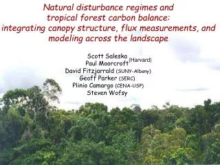
Natural disturbance regimes and tropical forest carbon balance: integrating canopy structure, flux measurements, and modeling across the landscape. Scott Saleska Paul Moorcroft David Fitzjarrald (SUNY-Albany) Geoff Parker (SERC) Plinio Camargo (CENA-USP) Steven Wofsy. (Harvard).

(Harvard)
E N D
Presentation Transcript
Natural disturbance regimes and tropical forest carbon balance: integrating canopy structure, flux measurements, and modeling across the landscape Scott SaleskaPaul MoorcroftDavid Fitzjarrald (SUNY-Albany)Geoff Parker (SERC) Plinio Camargo (CENA-USP)Steven Wofsy (Harvard)
Prior results I: eddy flux measurement show net loss of C in Tapajos National forest of Amazônia, attributable to recent disturbance event(s) 6 5 4 3 2 1 0 -1 -2 loss to atmosphere Accumulated Mg(C) ha-1 uptake Source: Saleska et al. (2003) Science 2001 2002 2003
25 20 15 10 5 0 -5 -10 -15 -20 -25 Modeled flux following disturbance in gap of a “balanced-biosphere” Amazon rainforest npp = net primary productivity (uptake)rh = heterotrophic respiration (loss) nep = net ecosystem productivity (change in carbon balance) Positive productivity (=uptake from atm) Mg (C) ha-2 yr-1 Note ecological sign convention! Negative productivity (=loss to atm) Gap Age (time since disturbance in years) Source: Moorcroft, Hurtt & Pacala (2001)
25 20 15 10 5 0 -5 -10 -15 -20 -25 Modeled flux following disturbance in gap of a “balanced-biosphere” Amazon rainforest npp = net primary productivity (uptake)rh = heterotrophic respiration (loss) nep = net ecosystem productivity (change in carbon balance) Positive productivity (=uptake from atm) Mg (C) ha-2 yr-1 Note ecological sign convention! Negative productivity (=loss to atm) Tapajos Km 67 site?(loss) Gap Age (time since disturbance in years) Source: Moorcroft, Hurtt & Pacala (2001)
25 Extrapolating measurements to landscape or region requires knowing: 20 15 10 5 0 • where measurement sites fall on this graph • frequency distribution of gap ages across the landscape -5 -10 -15 -20 -25 Modeled flux following disturbance in gap of a “balanced-biosphere” Amazon rainforest Mg (C) ha-2 yr-1 Note ecological sign convention! Tapajos Km 67 site?(loss) Gap Age (time since disturbance in years) Source: Moorcroft, Hurtt & Pacala (2001)
25 Extrapolating measurements to landscape or region requires knowing: 20 15 10 5 0 • where measurement sites fall on this graph • frequency distribution of gap ages across the landscape -5 selection bias towards pristine-looking sites?(uptake) -10 -15 -20 -25 Modeled flux following disturbance in gap of a “balanced-biosphere” Amazon rainforest Mg (C) ha-2 yr-1 Note ecological sign convention! Tapajos Km 67 site?(loss) Gap Age (time since disturbance in years) Source: Moorcroft, Hurtt & Pacala (2001)
Poses hard question: how to reliably estimate C-balance at large spatial scales Requirements: • Model that links disturbance state and forest carbon balance • Measurements of forest disturbance state to constrain model at large scales • Ability to testforest structure-constrained model predictions at points distributed across landscapes/regions
A. Modeling: the Ecosystem Demography (ED) Model • Plant community dynamics • carbon and nitrogen biogeochemistry • Explicit representation of size- and age-structure of ecosystem heterogeneity (Moorcroft, Hurtt and Pacala, 2001; Medvigy et al., 2004)
ED simulations relating forest size and age structure to carbon balance: Max canopy heightand … Tapajos National Forest
ED simulations relating forest size and age structure to carbon balance: Max canopy height and … Net Ecosystem Production (NEP) Tapajos National Forest
B. Measurements of forest disturbance state (as embodied in canopy structure) Aircraft-based Lidar gives canopy structure(at landscape scale) Source: Hurtt et al. (2004)
B. Measurements of forest disturbance state (as embodied in canopy structure) Ground-based Lidar gives canopy structure (local scale) km 67 tower site, July 2003 height (m) distance along transect (m) Source:Fitzjarrald & Parker, personal communication
Ground-based Lidar km 67 tower site, July 2003 height (m) distance along transect (m) Source:Fitzjarrald & Parker, personal communication
Future Work (2). Observations over larger spatial scales Ground-based Lidar km 67 tower site, July 2003 height (m) distance along transect (m) Source:Fitzjarrald & Parker, personal communication Gap fraction (canopy < 10 m) 25% height (m) fraction
C. Testingmodel predictions across landscape 10 km Question: What is the range of disturbance across the landscape scale in the Tapajos National Forest?
C. Testingmodel predictions across landscape 10 km 20 ha of biometry transects in tower footprint estab- lished 1999 Question: What is the range of disturbance across the landscape scale in the Tapajos National Forest? Km 67 tower Tapajos National Forest region, central eastern Amazônia
C. Testingmodel predictions across landscape 10 km 25m 15m 500m 0m 1000m 1500m 2000m 2500m 20 ha of biometry transects in tower footprint estab- lished 1999 Question: What is the range of disturbance across the landscape scale in the Tapajos National Forest? Km 67 tower T1 Km 72 T2 40 ha of new Transectsat Km72 (T1 & T2) and Km117 (T3 & T4) estab-lishedsummer 2003 T3 Km 117 T4 Tapajos National Forest region, central eastern Amazônia
C. Testingmodel predictions across landscape 10 km 20 ha of biometry transects in tower footprint estab- lished 1999 Question: What is the range of disturbance across the landscape scale in the Tapajos National Forest? Km 67 T1 Km 72 T2 • Large-scale Observations: • Live aboveground biomass • Vines • Coarse Woody Debris • Soil characteristics • Canopy structure (via ground-based Lidar) • Remote-sensing Lidar campaign (airborne LVIS, airborne Lidar or IceSat data) 40 ha of new Transectsat Km72 (T1 & T2) and Km117 (T3 & T4) estab-lishedsummer 2003 At spatially-distrib-uted transects T3 Km 117 T4 Spatially continuous in 20 x 60 km box Tapajos National Forest region, central eastern Amazônia
(A) ED model(includes canopy structure) Flux-Age relation Mg (C) ha-2 yr-1 Gap Age (time since disturbance in years) Age-Height Relation Gap Age Canopy Height (Moorcroft, et al., 2001)
(A) ED model(includes canopy structure) (B) Observation:canopy height distribution Flux-Age relation Mg (C) ha-2 yr-1 Height Gap Age (time since disturbance in years) Age-Height Relation Tree Density Gap Age Canopy Height (Moorcroft, et al., 2001)
(A) ED model(includes canopy structure) (B) Observation:canopy height distribution Flux-Age relation Mg (C) ha-2 yr-1 Model prediction:carbon balanceacross landscape Height Gap Age (time since disturbance in years) Age-Height Relation Tree Density Gap Age Canopy Height (Moorcroft, et al., 2001)
(A) ED model(includes canopy structure) (B) Observation:canopy height distribution Flux-Age relation Mg (C) ha-2 yr-1 Model prediction:carbon balanceacross landscape Height Gap Age (time since disturbance in years) Age-Height Relation Tree Density (C) Carbon Flux Observations Gap Age • Eddy fluxes (over time) • Landscape-scale plots(over space) Canopy Height (Moorcroft, et al., 2001) Test
ED Km 67 Initial Results(and one big caveat) Canopy Height Distribution Height (m) fraction
ED Km 67 Initial Results(and one big caveat) Canopy Height Distribution Large-scale sites (km 72 & km 117) Height (m) fraction
Loss | gain ED Km 67 Initial Results(and one big caveat) Corresponding ED-predicted Fluxes(95% confidence intervals from bootstrapping height data) Canopy Height Distribution Carbon Uptake (MgC/ha/yr Large-scale sites (km 72 & km 117) Height (m) Km67 Km72 km117site fraction
Loss | gain ED Km 67 Initial Results(and one big caveat) Corresponding ED-predicted Fluxes(95% confidence intervals from bootstrapping height data) Canopy Height Distribution eddy flux C-balance range Carbon Uptake (MgC/ha/yr Large-scale sites (km 72 & km 117) Height (m) biometry C-balance range Km67 Km72 km117site fraction
The caveat: scale used for LIDAR data aggregation Bin-size, 10 m Gap width = 40m Height (m) Meters of transect
The caveat: scale used for LIDAR data aggregation Bin-size, 20 m Gap width = 20m Height (m) Meters of transect
The caveat: scale used for LIDAR data aggregation Km 67 LIDAR data only Height (m) Baseline km67 data (horiz bin=2m) fraction
The caveat: scale used for LIDAR data aggregation Km 67 LIDAR data only Height (m) 4m bin Baseline km67 data (horiz bin=2m) fraction
The caveat: scale used for LIDAR data aggregation Km 67 LIDAR data only Height (m) 10m bin 4m bin Baseline km67 data (horiz bin=2m) fraction
The caveat: scale used for LIDAR data aggregation Km 67 LIDAR data only 20m bin Height (m) 10m bin 4m bin Baseline km67 data (horiz bin=2m) fraction
Loss | gain The caveat: scale used for LIDAR data aggregation LIDAR-constrained ED prediction Km 67 LIDAR data only 20m bin 10m bin 20m bin Carbon Uptake (MgC/ha/yr 4m bin Height (m) 10m bin 4m bin Baseline km67 data (horiz bin=2m) fraction LIDAR horiz bin width
Loss | gain The caveat: scale used for LIDAR data aggregation LIDAR-constrained ED prediction Km 67 LIDAR data only 20m bin 10m bin 20m bin Scale of ED model Carbon Uptake (MgC/ha/yr 4m bin Height (m) 10m bin 4m bin Baseline km67 data (horiz bin=2m) fraction LIDAR horiz bin width
Loss | gain Future work • Incorporate CWD explicitly into ED model: Current ED Carbon Uptake (MgC/ha/yr Patch Age (yrs)
Loss | gain Future work • Incorporate CWD explicitly into ED model: Current ED Expected effect of CWD module: smooth out decomp losses Carbon Uptake (MgC/ha/yr Patch Age (yrs)
Loss | gain Future work • Incorporate CWD explicitly into ED model: Current ED Less loss early Expected effect of CWD module: smooth out decomp losses Carbon Uptake (MgC/ha/yr More loss late Patch Age (yrs)
Conclusions • LIDAR detects variation in canopy structure across the landscape (km 67 different from km’s 72 and 117). • ED model can map LIDAR-detected canopy structure to distribution of patch age, and thence to carbon balance; and it predicts significantly different balances across the landscape • ED model-predicted fluxes are highly sensitive to spatial scale of LIDAR-data aggregation: key to match spatial scale of LIDAR data to scale of model • When the scales of observation and model are matched, the modeled carbon balance does not agree with observed balance at km67 • incorporation of CWD in ED model will likely improve the ability of ED to predict observed carbon balance.
Height (m) LAI (cm2/m2 in each 2m ht bins)
Km67 SAI(=Surface Area Index) is lower than LAI in ED ED mean LAI height Km67 mean SAI height
Effect of Aggregation on patchwise mean LAI height Aggregating SAI bins has no effect on mean, but narrows the distribution As distrib. narrows, lose high heights but these have similar positive fluxes to those just below 20 m bins Mean height 2m bins As distrib. narrows, lose lowest heights associated with big negative (loss) fluxes
o Max ht approach Mean SAI-ht approach LAI approach is less sensitive than max-ht. approach, but it is still scale-dependent.
10 km (B) Km 67 tower
10 km (B) Km 67 tower
10 km (B) Km 67 tower Km 83
(A) Km 67 T1 Km 72 T2 Km 83 10 km T3 Km 117 T4 (B) tower
(A) (B) tower Km 67 T1 Km 72 T2 Km 83 10 km (C) Center Path 25m 15m CWD Line 0m 500m 1000m 1500m 2000m 2500m DBH> 30 cm , dead or alive DBH> 10 cm, dead or alive, including lianas 0m 10m T3 Line Intercept CWD measure CWD > 7.5 cm DBH For CWD >30cm DBH, measure orientation Km 117 T4