Logistics Network Configuration
Logistics Network Configuration. Phil Kaminsky kaminsky@ieor.berkeley.edu. David Simchi-Levi Philip Kaminsky Edith Simchi-Levi. Outline. What is it? Methodology Modeling Data Aggregation Validation Solution Techniques Case Study: BuyPC.com. The Logistics Network.

Logistics Network Configuration
E N D
Presentation Transcript
Logistics Network Configuration Phil Kaminskykaminsky@ieor.berkeley.edu David Simchi-Levi Philip Kaminsky Edith Simchi-Levi
Outline • What is it? • Methodology • Modeling • Data Aggregation • Validation • Solution Techniques • Case Study: BuyPC.com
The Logistics Network The Logistics Network consists of: • Facilities:Vendors, Manufacturing Centers, Warehouse/ Distribution Centers, and Customers • Raw materials and finished products that flow between the facilities.
Customers, demand centers sinks Field Warehouses: stocking points Sources: plants vendors ports Regional Warehouses: stocking points Supply Inventory & warehousing costs Production/ purchase costs Transportation costs Transportation costs Inventory & warehousing costs
Decision Classifications • Strategic Planning: Decisions that typically involve major capital investments and have a long term effect • Determination of the number, location and size of new plants, distribution centers and warehouses • Acquisition of new production equipment and the design of working centers within each plant • Design of transportation facilities, communications equipment, data processing means, etc.
Decision Classifications • Tactical Planning: Effective allocation of manufacturing and distribution resources over a period of several months • Work-force size • Inventory policies • Definition of the distribution channels • Selection of transportation and trans-shipment alternatives
Decision Classifications • Operational Control: Includes day-to-day operational decisions • The assignment of customer orders to individual machines • Dispatching, expediting and processing orders • Vehicle scheduling
Network Design: Key Issues • Pick the optimal number, location, and size of warehouses and/or plants • Determine optimal sourcing strategy • Which plant/vendor should produce which product • Determine best distribution channels • Which warehouses should service which customers
Network Design: Key Issues The objective is to balance service level against • Production/ purchasing costs • Inventory carrying costs • Facility costs (handling and fixed costs) • Transportation costs That is, we would like to find a minimal-annual-cost configuration of the distribution network that satisfies product demands at specified customer service levels.
Network Design Tools:Major Components • Mapping • Mapping allows you to visualize your supply chain and solutions • Mapping the solutions allows you to better understand different scenarios • Color coding, sizing, and utilization indicators allow for further analysis • Data • Data specifies the costs of your supply chain • The baseline cost data should match your accounting data • The output data allows you to quantify changes to the supply chain • Engine • Optimization Techniques
Data for Network Design 1. A listing of all products 2. Location of customers, stocking points and sources 3. Demand for each product by customer location 4. Transportation rates 5. Warehousing costs 6. Shipment sizes by product 7. Order patterns by frequency, size, season, content 8. Order processing costs 9. Customer service goals
Too Much Information Customers and Geocoding • Sales data is typically collected on a by-customer basis • Network planning is facilitated if sales data is in a geographic database rather than accounting database 1. Distances 2. Transportation costs • New technology exists for Geocoding the data based on Geographic Information System (GIS)
Aggregating Customers • Customers located in close proximity are aggregated using a grid network or clustering techniques. All customers within a single cell or a single cluster are replaced by a single customer located at the centroid of the cell or cluster.We refer to a cell or a cluster as a customer zone.
Impact of Aggregating Customers • The customer zone balances • Loss of accuracy due to over aggregation • Needless complexity • What effects the efficiency of the aggregation? • The number of aggregated points, that is the number of different zones • The distribution of customers in each zone.
Why Aggregate? • The cost of obtaining and processing data • The form in which data is available • The size of the resulting location model • The accuracy of forecast demand
Recommended Approach • Use at least 300 aggregated points • Make sure each zone has an equal amount of total demand • Place the aggregated point at the center of the zone • In this case, the error is typically no more than 1%
Testing Customer Aggregation • 1 Plant; 1 Product • Considering transportation costs only • Customer data • Original Data had 18,000 5-digit zip code ship-to locations • Aggregated Data had 800 3-digit ship-to locations • Total demand was the same in both cases
Comparing Output Total Cost:$5,796,000 Total Customers: 18,000 Total Cost:$5,793,000 Total Customers: 800 Cost Difference < 0.05%
Product Grouping • Companies may have hundreds to thousands of individual items in their production line • Variations in product models and style • Same products are packaged in many sizes • Collecting all data and analyzing it is impractical for so many product groups
A Strategy for Product Aggregation • Place all SKU’s into a source-group • A source group is a group of SKU’s all sourced from the same place(s) • Within each of the source-groups, aggregate the SKU’s by similar logistics characteristics • Weight • Volume • Holding Cost
Within Each Source Group, Aggregate Products by Similar Characteristics Rectangles illustrate how to cluster SKU’s.
Test Case for Product Aggregation • 5 Plants • 25 Potential Warehouse Locations • Distance-based Service Constraints • Inventory Holding Costs • Fixed Warehouse Costs • Product Aggregation • 46 Original products • 4 Aggregated products • Aggregated products were created using weighted averages
Sample Aggregation Test:Product Aggregation Total Cost:$104,564,000 Total Products: 46 Total Cost:$104,599,000 Total Products: 4 Cost Difference: 0.03%
Transport Rate Estimation • Huge number of rates representing all combinations of product flow • An important characteristic of a class of rates for truck, rail, UPS and other trucking companies is that the rates are quite linear with the distance.
Transport Rate Estimation Source: Ballou, R. H. Business Logistics Management
Industry Benchmarks:Transportation Costs • Transportation Rates (typical values) • Truck Load: $0.10 per ton-mile • LTL: $0.31 per ton-mile • Small Package: 3X LTL rates- more for express • Rail: 50-80% of TL rates
LTL Freight Rates • Each shipment is given a class ranging from 500 to 50 • The higher the class the greater the relative charge for transporting the commodity. • A number of factors are involved in determining a product’s specific class. These include • Density • Ease or difficulty of handling • Liability for damage
Basic Freight Rates • With the commodity class and the source and destination Zip codes, the specific rate per hundred pound can be located. • This can be done with the help of CZAR, Complete Zip Auditing and Rating, which is a rating engine produced by Southern Motor Carriers. • Finally to determine the cost of moving commodity A from City B to City C, use the equation weight in cwt rate
Other Issues • Mileage Estimation • Street Network • Straight line distances • This is of course an underestimate of the road distance. To estimate the road distance we multiply the straight line distance by a scale factor, . Typically =1.3.
Other Issues • Future demand • Facility costs • Fixed costs; not proportional to the amount of material the flows through the warehouse • Handling costs; labor costs, utility costs • Storage costs; proportional to the inventory level • Facilities capacities
Customers, demand centers sinks Field Warehouses: stocking points Sources: plants vendors ports Regional Warehouses: stocking points Supply Inventory & warehousing costs Production/ purchase costs Transportation costs Transportation costs Inventory & warehousing costs
Minimize the cost of your logistics network without compromising service levels Optimal Number of Warehouses
The Impact of Increasing the Number of Warehouses • Improve service level due to reduction of average service time to customers • Increase inventory costs due to a larger safety stock • Increase overhead and set-up costs • Reduce transportation costs in a certain range • Reduce outbound transportation costs • Increase inbound transportation costs
Industry Benchmarks:Number of Distribution Centers Food Companies Chemicals Pharmaceuticals Avg. # of WH 3 14 25 - High margin product - Service not important (or easy to ship express) - Inventory expensive relative to transportation - Low margin product - Service very important - Outbound transportation expensive relative to inbound Sources: CLM 1999, Herbert W. Davis & Co; LogicTools
A Typical Network Design Model • Several products are produced at several plants. • Each plant has a known production capacity. • There is a known demand for each product at each customer zone. • The demand is satisfied by shipping the products via regional distribution centers. • There may be an upper bound on total throughput at each distribution center.
A Typical Location Model • There may be an upper bound on the distance between a distribution center and a market area served by it • A set of potential location sites for the new facilities was identified • Costs: • Set-up costs • Transportation cost is proportional to the distance • Storage and handling costs • Production/supply costs
Complexity of Network Design Problems • Location problems are, in general, very difficult problems. • The complexity increases with • the number of customers, • the number of products, • the number of potential locations for warehouses, and • the number of warehouses located.
Solution Techniques • Mathematical optimization techniques: • Exact algorithms: find optimal solutions • Heuristics: find “good” solutions, not necessarily optimal • Simulation models: provide a mechanism to evaluate specified design alternatives created by the designer.
Heuristics and the Need for Exact Algorithms • Single product • Two plants p1 and p2 • Plant P1 has an annual capacity of 200,000 units. • Plant p2 has an annual capacity of 60,000 units. • The two plants have the same production costs. • There are two warehouses w1 and w2 with identical warehouse handling costs. • There are three markets areas c1,c2 and c3 with demands of 50,000, 100,000 and 50,000, respectively.
Why Optimization Matters? $0 D = 50,000 $3 Cap = 200,000 $4 $5 $5 D = 100,000 $2 $4 $1 $2 Cap = 60,000 $2 D = 50,000 Production costs are the same, warehousing costs are the same
Traditional Approach #1:Assign each market to closet WH. Then assign each plant based on cost. D = 50,000 Cap = 200,000 $5 x 140,000 D = 100,000 $2 x 50,000 $1 x 100,000 $2 x 60,000 Cap = 60,000 $2 x 50,000 D = 50,000 Total Costs = $1,120,000
Traditional Approach #2:Assign each market based on total landed cost $0 D = 50,000 $3 Cap = 200,000 P1 to WH1 $3 P1 to WH2 $7 P2 to WH1 $7 P2 to WH 2 $4 $4 $5 $5 D = 100,000 $2 P1 to WH1 $4 P1 to WH2 $6 P2 to WH1 $8 P2 to WH 2 $3 $4 $1 $2 Cap = 60,000 $2 D = 50,000 P1 to WH1 $5 P1 to WH2 $7 P2 to WH1 $9 P2 to WH 2 $4
Traditional Approach #2:Assign each market based on total landed cost $0 D = 50,000 $3 Cap = 200,000 P1 to WH1 $3 P1 to WH2 $7 P2 to WH1 $7 P2 to WH 2 $4 $4 $5 $5 D = 100,000 $2 P1 to WH1 $4 P1 to WH2 $6 P2 to WH1 $8 P2 to WH 2 $3 $4 $1 $2 Cap = 60,000 $2 D = 50,000 P1 to WH1 $5 P1 to WH2 $7 P2 to WH1 $9 P2 to WH 2 $4 Market #1 is served by WH1, Markets 2 and 3 are served by WH2
Traditional Approach #2:Assign each market based on total landed cost $0 x 50,000 D = 50,000 $3 x 50,000 Cap = 200,000 P1 to WH1 $3 P1 to WH2 $7 P2 to WH1 $7 P2 to WH 2 $4 $5 x 90,000 D = 100,000 P1 to WH1 $4 P1 to WH2 $6 P2 to WH1 $8 P2 to WH 2 $3 $1 x 100,000 $2 x 60,000 Cap = 60,000 $2 x 50,000 D = 50,000 P1 to WH1 $5 P1 to WH2 $7 P2 to WH1 $9 P2 to WH 2 $4 Total Cost = $920,000