CONJUGATE GRADIENT METHOD
CONJUGATE GRADIENT METHOD. Monica Garika Chandana Guduru . METHODS TO SOLVE LINEAR SYSTEMS. Direct methods Gaussian elimination method LU method for factorization Simplex method of linear programming Iterative method Jacobi method Gauss-Seidel method

CONJUGATE GRADIENT METHOD
E N D
Presentation Transcript
CONJUGATE GRADIENT METHOD Monica Garika Chandana Guduru
METHODS TO SOLVE LINEAR SYSTEMS • Direct methods Gaussian elimination method LU method for factorization Simplex method of linear programming • Iterative method Jacobi method Gauss-Seidel method Multi-grid method Conjugate gradient method
Conjugate Gradient method • The CG is an algorithm for the numerical solution of particular system of linear equations Ax=b. Where A is symmetric i.e., A = AT and positive definite i.e., xT * A * x > 0 for all nonzero vectors If A is symmetric and positive definite then the function Q(x) = ½ x`Ax – x`b + c
Conjugate gradient method • Conjugate gradient method builds up a solution x*€ Rnin at most n steps in the absence of round off errors. • Considering round off errors more than n steps may be needed to get a good approximation of exact solution x* • For sparse matrices a good approximation of exact solution can be achieved in less than n steps in also with round off errors.
Practical Example In oil reservoir simulation, The number of linear equations corresponds to the number of grids of a reservoir • The unknown vector x is the oil pressure of reservoir • Each element of the vector x is the oil pressure of a specific grid of the reservoir
Linear System Unknown vector (what we want to find) Known vector Square matrix
Positive Definite Matrix [ x1 x2 … xn] > 0
Procedure • Finding the initial guess for solution 𝑥0 • Generates successive approximations to 𝑥0 • Generates residuals • Searching directions
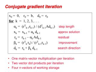
Conjugate gradient iteration • x0 = 0, r0 = b, p0 = r0 • for k = 1, 2, 3, . . . • αk = (rTk-1rk-1) / (pTk-1Apk-1) step length • xk= xk-1 + αk pk-1 approximate solution • rk = rk-1 – αk Apk-1 residual • βk = (rTkrk) / (rTk-1rk-1) improvement • pk= rk+ βk pk-1 search direction
Iteration of conjugate gradient method is of the form x(t) = x(t-1) + s(t)d(t) where, x(t) is function of old value of vector x s(t) is scalar step size x d(t) is direction vector Before first iteration, values of x(0), d(0) and g(0) must be set
Steps to find conjugate gradient method • Every iteration t calculates x(t) in four steps : Step 1: Compute the gradient g(t) = Ax(t-1) – b Step 2: Compute direction vector d(t) = - g(t) + [g(t)` g(t) / g(t-1)` g(t-1)] d(t-1) Step 3: Compute step size s(t) = [- d(t)` g(t)]/d(t)’ A d(t)] Step 4: Compute new approximation of x x(t) = x(t-1) + s(t)d(t)
Sequential Algorithm 1) 𝑥0 = 0 2) 𝑟0 := 𝑏 − 𝐴𝑥0 3) 𝑝0 := 𝑟0 4) 𝑘 := 0 5) 𝐾𝑚𝑎𝑥 := maximum number of iterations to be done 6) if 𝑘 < 𝑘𝑚𝑎𝑥 then perform 8 to 16 7) if 𝑘 = 𝑘𝑚𝑎𝑥 then exit 8) calculate 𝑣 = 𝐴𝑝k 9) αk : = rkTrk/pTk v 10) 𝑥k+1:= 𝑥k + akpk 11) 𝑟k+1 := 𝑟k − ak v 12) if 𝑟k+1 is sufficiently small then go to 16 end if 13) 𝛽k :=( r T k+1 r k+1)/(rTk 𝑟k) 14) 𝑝k+1 := 𝑟k+1 +βkpk 15) 𝑘 := 𝑘 + 1 16) 𝑟𝑒𝑠𝑢𝑙𝑡 = 𝑥k+1
Complexity analysis • To Identify Data Dependencies • To identify eventual communications • Requires large number of operations • As number of equations increases complexity also increases .
Why To Parallelize? • Parallelizing conjugate gradient method is a way to increase its performance • Saves memory because processors only store the portions of the rows of a matrix A that contain non-zero elements. • It executes faster because of dividing a matrix into portions
How to parallelize? • For example , choose a row-wise block striped decomposition of A and replicate all vectors • Multiplication of A and vector may be performed without any communication • But all-gather communication is needed to replicate the result vector • Overall time complexity of parallel algorithm is Θ(n^2 * w / p + nlogp)
Row wise Block Striped Decomposition of a Symmetrically Banded Matrix
Algorithm of a Parallel CG on each Computing Worker (cw) 1) Receive 𝑐𝑤𝑟0,𝑐𝑤 𝐴,𝑐𝑤 𝑥0 2) 𝑐𝑤𝑝0 =𝑐𝑤 𝑟0 3) 𝑘 := 0 4) 𝐾𝑚𝑎𝑥 := maximum number of iterations to be done 5) if 𝑘 < 𝑘𝑚𝑎𝑥 then perform 8 to 16 6) if 𝑘 = 𝑘𝑚𝑎𝑥 then exit 7) 𝑣 =𝑐𝑤 𝐴𝑐𝑤𝑝𝑘 8) 𝑐𝑤𝑁𝛼𝑘 9) 𝑐𝑤𝐷𝛼𝑘 10) Send 𝑁𝛼𝑘,𝐷𝛼𝑘 11) Receive 𝛼𝑘 12) 𝑥𝑘+1 = 𝑥𝑘 + 𝛼𝑘𝑝𝑘 13) Compute Partial Result of 𝑟𝑘+1: 𝑟𝑘+1 =𝑟𝑘 − 𝛼𝑘𝑣 14) Send 𝑥𝑘+1, 𝑟𝑘+1 15) Receive 𝑠𝑖𝑔𝑛𝑎𝑙 16) if 𝑠𝑖𝑔𝑛𝑎𝑙 = 𝑠𝑜𝑙𝑢𝑡𝑖𝑜𝑛𝑟𝑒𝑎𝑐ℎ𝑒𝑑 go to 23 17) 𝑐𝑤𝑁𝛽𝑘 18) 𝑐𝑤𝐷𝛽𝑘 19) Send 𝑐𝑤𝑁𝛽𝑘 , 𝑐𝑤𝐷𝛽𝑘 20) Receive 𝛽𝑘 21) 𝑐𝑤𝑝𝑘+1 =𝑐𝑤 𝑟𝑘+1 + 𝛽𝑘 𝑐𝑤𝑝𝑘 22) 𝑘 := 𝑘 + 1 23) Result reached
Speedup of Parallel CG on Grid Versus Sequential CG on Intel
We consider the difference between f at the solution x and any other vector p:
Parallel Computation Design • Parallel Computation Design • – Iterations of the conjugate gradient method can be executed • only in sequence, so the most advisable approach is to parallelize the computations, that are carried out at each iteration • The most time-consuming computations are the multiplication of matrix A by the vectors x and d • – Additional operations, that have the lower computational complexity order, are different vector processing procedures (inner product, addition and subtraction, multiplying by a scalar). • While implementing the parallel conjugate gradient method, it can be used parallel algorithms of matrix-vector multiplication,
T g d k k a = - k T d Qd k k T g Qd k+1 k b = k T d Qd k k “Pure” Conjugate Gradient Method (Quadratic Case) 0 - Starting at any x0define d0 = -g0 = b - Q x0 , where gk is the column vector of gradients of the objective function at point f(xk) 1 - Using dk , calculate the new point xk+1= xk+ akdk , where 2 - Calculate the new conjugate gradient direction dk+1, according to: dk+1= - gk+1+ bkdk where
ADVANTAGES Advantages: • 1) Gradient is always nonzero and linearly independent of all previous direction vectors. • 2) Simple formula to determine the new direction. Only slightly more complicated than steepest descent. • 3) Process makes good progress because it is based on gradients.
ADVANTAGES • Attractive are the simple formulae for updating the direction vector. • Method is slightly more complicated than steepest descent, but converges faster. • Conjugate gradient method is an Indirect Solver • Used to solve large systems • Requires small amount of memory • It doesn’t require numerical linear algebra
Conclusion • Conjugate gradient method is a linear solver tool which is used in a wide range of engineering and sciences applications. • However, conjugate gradient has a complexity drawback due to the high number of arithmetic operations involved in matrix vector and vector-vector multiplications. • Our implementation reveals that despite the communication cost involved in a parallel CG, a performance improvement compared to a sequential algorithm is still possible.
References • Parallel and distributed computing systems by Dimitri P. Bertsekas, John N.Tsitsiklis • Parallel programming for multicore and cluster systems by Thomas Rauber,GudulaRunger • Scientific computing . An introduction with parallel computing by Gene Golub and James M.Ortega • Parallel computing in C with Openmp and mpi by Michael J.Quinn • Jonathon Richard Shewchuk, ”An Introduction to the Conjugate Gradient Method Without the Agonizing Pain”, School of Computer Science, Carnegie Mellon University, Edition 1 1/4