Download
1 / 78
780 likes | 918 Vues
Practical use of Screen Space Ambient Occlusion. Michał Drobot Visual Technical Director Reality Pump. Talk Outline. Motivation Theory General Idea Practical Solution in Details Screen Space to Camera Space Raycasting Blocker Test Filtering Compositing with HDRi. Talk Outline.

E N D
Practical use of Screen Space Ambient Occlusion Michał Drobot Visual Technical Director Reality Pump
Talk Outline • Motivation • Theory • General Idea • Practical Solution in Details • Screen Space to Camera Space • Raycasting • Blocker Test • Filtering • Compositing with HDRi
Talk Outline • Tackling Problems • Deffered Renderers • Forward Renderers • Performance & IQ Optimizations • Further Development • Summary • Questions?
Motivation • Multiplatform • HQ seamless land/city-scape rendering • Realistic lighting model: • Dynamic day cycle • Dynamic lights • Dynamic environments • Global Illumination Approximation - taking into consideration all above = PROBLEMATIC!
Motivation • Solutions: • PRT – maps • Per Vertex SH • Point Clouds • Inhouse off-line solutions… • All failed: • Memory consumption (X360) • Performance • Flexibility
Motivation • Needed new solution • Dynamic • Scalable • Max Performance/Memory ratio • Screen Space Solution • Image Depth enhacement publications • Hybrid rendering engine • Z-based post processing
Theory • Ambient Occlusion – Technically • Global Illumination approximation • Omnidirectional lighting • Accessiblity shading • Film Industry proven prepass Skylight
Theory • AO – visual appeal • Artists using Skylight bake in textures • Enviromental effect – surface reaction to: • Dirt/weathering • Light • Prepass for Global Illumination • Enhances scene by depth, curvature, spatial proximity clues
Theory • Integral of blocker function over the hemisphere
Theory • Point A is not occluded • Point B is darkened (high geo. Proximity)
General Idea • Screen Space = simplified calculation domain (performance) • Depth buffer • Resembles scene in SS • Generally available • Preferably linear - high precision (>FP16) • Pixel (x,y) in SS & DB val = (x,y,z) in CS • Camera Space = simplified calculation domain (complexity)
Theory • For each pixel in SS • For 1 to N samples • Transform to CS domain • Raycast in CS in random direction on point’s normal hemisphere • Gather irradiance information from surface hit check • Cumulate results considering atmosphere attenuation, radiance energy • Return resulting irradiance • Composite final SS result layer with HDRi
Screen Space to Camera Space • SS pixel (x,y) & depth value = (x,y,z) in CS • Min 1 mul = fast • Keep your depth high precision to avoid artifacts • Preferable 32FP linear depth (depends on your scene depth range) • Our solution is based on 16FP linear depth transformed from original log Depth Buffer (gives filterable artifacts)
Raycasting • Raycast by raymarch • Generate normalized hemisphere of randomly distributed points with uniform distribution ie. Poisson • Rotate hemisphere so its’ horizon is perpendicular to point’s normal (for now we assume to have it) • Scale the hemisphere for desired effect range • Offset CS original point by generated points
Raycast Transform new point from CS to SS • Acquire points z value from our scene in SS • We can also acquire additional info like diffuse color, radiance energy etc.
Blocker Test • In the same domain we’ve got • Depth of ‘possible’ hit (pd) • Real depth at (x,y) of ‘possible’ hit point (rd) • We want to check if we hit something with our ray • If something exists in our depth buffer at SS cordinates of ‘pd’ and at the same depth we’ve got a HIT
Blocker Test • We need a comparision function considering attenuation, limited samples, possible precision errors • Real Distance Proximity Evaluation • Depth Difference Evaluation
Blocker Test (RDPE) • Real Distance Proximity Evaluation (RDPE) • Abs(pd-rd) < E • If TRUE = HIT • Accumulate results - Occlusion += 1/(1+(length(ray)*scale)^2) • If FALSE = miss • Discard results – SamplesNo--; • Alternativly for high accuracy repeat whole process of raycasting using linear/binary search • finalOcclusion = Occlusion/SamplesNo
Blocker Test (RDPE) • Pros • conceptualy precise results • Superb quality with linear/binary raymarching (matching offline renderers) • Ideal for GI • Global (full screen) solution • Cons • Discarding MISSes leads to undersampling, requiring more sample with good distribution • Requires ray length calculations • Insane sampling rate with raymarching solution: SampleNo * PerSampleMissSampling
Blocker Test (RDPE) • Scaleability • E – Epsilon / Sample No Ratio • Iteration/E limit for raymarching • Still Raymarched solution needs at least 16 subsamples on avg (using flow control) • Practically useless due to undersampling artifacts while using sane number of samples
Blocker Test (DDE) • Depth Difference Evaluation (DDE) • Use all depth difference data with atennuation function • Occlusion = 1.0/(1.0+ (pd – rd)^2) • FinalOcclusion = Occlusion/SamplesNo
Blocker Test (DDE) • Pros • Fast • Simple • Perceptually accurate • Cons • Lacks accuracy • Gives more local results • Generally too local for GI
Blocker Test (DDE) • Scaleability • Sample rate tweaking • Scale samples with Z – depth (flow control) • Practically DDE is a WIN • But… only for this generation…
Filtering • Acquired Occlusion layer due to undersampling artifacts should be filtered • Due to AO low-frequency nature denoise blurring filters are the weapon of choice • Should smooth out results, denoise the signal and retain the details
Filtering • Gaussian Filter • Weighted average of sampled values • Requires preprocessed kernel weights • Kernel of NxN pixels
Filtering • Gaussian Filter • 2 pass filtering with interpolator usage • Very fast O(N) • Good smooth and denoise ability • Removes details, blurs edges • AO bleeding occurs • Introduces new artifacts (halos, bleeding)
Filtering Gaussian 18x18 Separable 18 taps
Filtering • Median filter • Median of sampled values • Kernel of NxN pixels • Heavy use of vector arithmetics for value sorting
Filtering • Median filter • 1 pass artifact free filter is O(N^2) • That’s too slow for reasonable kernel size • Possible use of combined multipass filters of small size • IQ better than gaussian, but too slow • 2 pass (V/H) is only O(2*N) • Fast enough • Not correct • May Introduces block artifacts • Usable as multipass/varied kernel size filter
Filtering Median 18x18 Separable 18 taps
Filtering Median 2x(6x6) Non Separable 18 taps
Filtering • Bilateral filtering • 3D filter • Filtering in domain of spatial proximity and intensity • Possible fast implementation using vector artihmetics BF[I]p = (1/Wp)Sum[q e S]( G[d](||p-q||)*G[i](|Ip-Iq)*Iq)
Filtering • We can simplify BF using same Gaussian for proximity and intensity domains • For each pixel p • Normalize Sum of • For each pixel q e S • Gaussian(||p-q||) * Gaussian(|Ip-Iq|) * Iq
Filtering • Bilateral filter is NOT separable • But results of separable filtering are acceptable • We can use linear filtering for bigger kernels • Optimized BF is O(n) and as fast as gaussian when done right
Filtering Bilateral 18x18 Separable 18 taps
Filtering Bilateral 9x9 Separable 18 taps
Filtering • Bilateral Filter • Gives very good smoothing • Retains details • Doesn’t affect edges • Prevents bleeding • Is fast • Is our choice
Filtering Original Gaussian 18x18 Bilateral 18x18 Median 2x(6x6) Median 9x9 Bilateral 9x9
Compositing with HDRi • Forward rendering • Compose as post process by multiply with HDRi before tone mapping • Exposure will need adjustement • Post HDR – AP soft light layer processing (or other chosen by artists) • Deffered rendering • Do it first • Use it as ambient occlusion term during material shading and lighting pass