SUMA
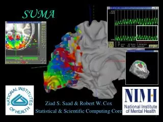
SUMA. Statistical & Scientific Computing Core. SUMA. SUrface MApping with AFNI. Surface mapping & viewing program tightly linked to AFNI Complements AFNI’s slice and volume rendering modes Provides a framework for fast and user-customizable surface based analysis


SUMA
E N D
Presentation Transcript
SUMA Statistical & Scientific Computing Core
SUrface MApping with AFNI • Surface mapping & viewing program tightly linked to AFNI • Complements AFNI’s slice and volume rendering modes • Provides a framework for fast and user-customizable surface based analysis • Supports surface models created by: FreeSurfer http://surfer.nmr.mgh.harvard.edu SureFit/Caret http://stp.wustl.edu/resources/display.html BrainVoyager http://www.brainvoyager.com • Allows representation of sparsely defined 3D data
System requirements MESA Library 4.0.1 (an API closely resembling OpenGL) http://www.mesa3d.org • Currently Running On: • Centrino, 1.4 Ghz / Linux • 1Gb RAM • nVIDIA GeForce4 graphics card 64 Mb • Also Runs On: • SGI • SUN with openGL 1.2 or newer • Mac OSX with Xfree86, Motif and Mesa
Installation • Binaries for SUMA are available from: http://afni.nimh.nih.gov/ssc/ziad/SUMA/SUMA_DownloadTable.htm • On some machines (i.e. Linux), SUMA should be compiled locally for optimal performance. • To compile SUMA you need to have: • Motif (both libraries and header files) • Mesa (OpenGL) • AFNI’s source code distribution • Detailed installation info for various systems: http://afni.nimh.nih.gov/ssc/ziad/SUMA/SUMA_Installation.htm
Where do surface models come from ? • For surface based analysis: • Must create surfaces for individual subjects • PreSUMA: • Collect, align and average high-quality, high-resolution anatomical data • On NIMH’s 3T-1, 4 MPRAGE data sets will do • Correct image non-uniformity • Using AFNI’s 3dUniformize or the N3 normalization tool [J.G. Sled et al. 98] • Create and correct surfaces • Using FreeSurfer, SureFit or BrainVoyager • CircumSUMA: • Align surface with experimental data • Using @SUMA_AlignToExperiment • Map experimental volumetric data to surface • Using AFNI and SUMA • PostSUMA: • Fame, Fortune and Fortitude for some, if not all, or none of you
Where do surface models come from ? • For display (mostly) of Talairach data: • Use the Talairach surfaces created from the N27 brain data set using FreeSurfer. • Ready to use, no surface creation or alignment needed.
What’s a surface made of? Node Edge
A: Preparing surface models for SUMA Create Surface Models (FreeSurfer, SureFit, etc.) High-Res. Anatomical MRI data @SUMA_Make_Spec_FS @SUMA_Make_Spec_SF Spec File ASCII file defining relationships between different surfaces SurfVol AFNI-format Surface Volume that is aligned with surface models
A: Preparing surface models for SUMA • Create the Surface Volume • SurfVol is an AFNI data set created from data used to create the surfaces. • Create the surface specifications (spec) file • The Spec file defines the relationships between the different surfaces. • Both the surface volume and the Spec file are created automatically • Using @SUMA_Make_Spec_FS for FreeSurfer surfaces • Using @SUMA_Make_Spec_SF for SureFit surfaces • At this point, surface models should be in excellent alignment with SurfVol • Use SUMA to verify alignment • Scroll through the volume to make sure surfaces are accurate • Check especially for inferior temporal and occipital areas
A: Preparing surface models for SUMA • Demo for FreeSurfer surfaces: • cd suma_demo/SurfData • This is where FreeSurfer’s directories reside • @SUMA_Make_Spec_FS -sid DemoSubj • Creates the SurfVol from the .COR files • DemoSubj_SurfVol+orig • Creates ASCII versions of surfaces found in the surf directory • lh*.asc and rh*.asc (if rh surfaces are provided) • Creates he Spec files for the left and right hemisphere surfaces • DemoSubj_lh.spec and DemoSubj_rh.spec (if rh surfaces are provided) • cd SUMA • afni –niml & • launches AFNI to allow the viewing of DemoSubj_lh.spec • the –niml option tells AFNI to listen to connections from SUMA • suma –spec DemoSubj_lh.spec –sv DemoSubj_SurfVol+orig • or execute the script: ./run_suma Hands-On
Check for proper alignment and defects • With both SUMA and AFNI running • Press ‘t’ in the suma window to establish a connection to AFNI and send the mapping reference surface(s). • If you open the surface volume in AFNI, you should see the surface overlaid on top of it. • Switch Underlay to DemoSubj_SurfVol+orig and open an axial view. You will see a trace of the intersection of the surface with the anatomical slices displayed. • You could also see boxes representing the nodes that are within +/- 1/2slice from the center of the slice in view. • Colors and node box visibility can be changed to suit your fancy from the Control Surface button in AFNI. • Navigate through the volume in AFNI. • make sure you have an excellent alignment between volume and surface • make sure surface adequately represents areas of the brain that are difficult to segment • occipital cortex • inferior frontal and inferior temporal regions Hands-On
Check for proper alignment and defects Note: Viewed without the volume underlay, it is extremely difficult to tell if surface models with no topological defects accurately represent the cortical surface. • The Surface Volume and the surfaces must be in perfect alignment. • If you have an improper alignment, it should be addressed here. • This should not happen for FreeSurfer and SureFit surfaces created in the standard fashion. • Watch for error messages and warnings that come up in the shell as the surfaces are read in. These messages should be screened once since they do not change unless the surface’s geometry or topology is changed. Hands-On
Basic SUMA viewer functions • Rotating the surface: • Mouse button-1: keep it down while moving the mouse left to right. This rotates the surface about the screen's Y-axis (dotted green). Let go of button-1. • Repeat with up and down motion for rotation about X-axis and motion in various directions for rotations mimicking those of a trackball interface. • Also try up/down/left/right arrow keys. • Arrow keys rotate by increments specified by the environment variable: SUMA_ArrowRotAngle (degrees). Hands-On
Basic SUMA viewer functions • Translating the surface: • Mouse button-2: keep it down while moving the mouse to translate surface along screen X and Y axes or any combinations of the two. • Also try shift+arrow keys. • Zooming in/out: • Both buttons 1&2 or Shift + button 2: while pressing buttons, move mouse down or up to zoom in and out, respectively. • Also try keyboard buttons 'Z' and 'z' for zooming in and out, respectively. Hands-On
Basic SUMA viewer functions • Cardinal views: • ctrl + Left/Right: Views along LR axis • ctrl + Up/Down: Views along SI axis • ctrl + shift + Up/down: Views along AP axis • Resetting the view point: • Press Home to get back to the original vantage point. • Using momentum feature: • Press ‘m’ to toggle momentum on. Click the left mouse button and release the button as you are dragging the mouse. Hands-On
Basic SUMA viewer functions • Picking a Node or Facet: • Mouse button 3: press over a location on a surface to pick the closest facet and node to the location of the pointer. • The closest node is highlighted with a blue sphere • The closest facet is highlighted with a gray triangle • Note the information written to the shell regarding the properties of the picked Node and Facet. • When connected to AFNI (after having pressed ‘t’), watch the AFNI crosshair jump to the corresponding location in the volume. • Conversely, position the crosshair in AFNI (left click) at a position close to the surface and watch the crosshair relocate in SUMA. • You can swap button 1 & 3’s functions using the environment variable: SUMA_SwapButtons_1_3 Hands-On
world AFNI SUMA world • AFNI and SUMA are independent programs and communicate using NIML formatted data elements • via shared memory if both programs are on the same computer • via network sockets otherwise • Both AFNI and SUMA can also communicate with other programs • NIML: NeuroImaging Markup Language developed by Dr. R.W. Cox • NIML will be the main format for SUMA’s data storage. • NIML API library for packing/unpacking data is available and documented. • Communication protocol allows any independent program to communicate with AFNI. • Advantages include: • Programs execute on separate machines • Fast development • Screen real-estate • Blemishes include: • Only one AFNI can be listening for connections • Only one SUMA can connect to AFNI
Relationships between surface models • Surface Geometry: • refers to the spatial coordinates of the nodes forming the surface model • Surface Topology: • refers to the connectivity between nodes forming the surface model • Models with different geometry but similar topology are created for each surface model. • white/grey, pial, inflated, spherical, flattened, etc. • Some models’ geometries are anatomically correct • Pial and/or white matter surfaces can be used for relating to volume data. • Inflated, flattened and spherical cannot be directly linked to volume data. The link is done via their corresponding anatomically-correct surfaces.
SmoothWm Inflated Spherical Inflated, Occipital cut Pial Overlay of anatomically correct Pial and SmoothWm surfaces over anatomical volume Flattened, Occipital cut
# delimits comments# define the group Group = DemoSubj# define various States StateDef = smoothwm StateDef = pial StateDef = inflated NewSurface SurfaceFormat = ASCII SurfaceType = FreeSurfer FreeSurferSurface = lh.smoothwm.asc LocalDomainParent = SAME SurfaceState = smoothwm EmbedDimension = 3NewSurface SurfaceFormat = ASCII SurfaceType = FreeSurfer FreeSurferSurface = lh.pial.asc LocalDomainParent = lh.smoothwm.asc SurfaceState = pial EmbedDimension = 3 Sample Spec File NewSurface SurfaceFormat = ASCII SurfaceType = FreeSurfer FreeSurferSurface = lh.inflated.asc LocalDomainParent = lh.smoothwm.asc SurfaceState = inflated EmbedDimension = 3NewSurface SurfaceFormat = ASCII SurfaceType = FreeSurfer FreeSurferSurface = lh.sphere.asc LocalDomainParent = lh.smoothwm.asc SurfaceState = sphere EmbedDimension = 3 Hands-On
Details of the Spec file: • The Spec file contains information about the surfaces that will be viewed. • Information is specified in the format: field = value. • The = sign must be preceded and followed by a space character. • # delimit comment lines, empty lines and tabs are ignored. • In addition to fields, there is also the NewSurface tag which is used to announce a new surface. • Unrecognized text will cause the program parsing Spec file to complain and exit. Hands-On
Details of the Spec file: • The fields are: • Group: Usually the Subject's ID. In the current SUMA version, you can only have one group per spec file. All surfaces read by SUMA must belong to a group. • FreeSurferSurface: Name of the FreeSurfer surface. • SurfaceFormat: ASCII or BINARY • SurfaceType: FreeSurfer or SureFit • SurfaceState: Surfaces can be in different states such as inflated, flattened, etc. The label of a state is arbitrary and can be defined by the user. The set of available states must be defined with StateDef at the beginning of the Spec file. Hands-On
Details of the Spec file: • The fields are: • StateDef: Used to define the various states. This must be placed before any of the surfaces are specified. • Anatomical: Used to indicate whether surface is anatomically correct (Y) or not (N). • LocalDomainParent: Name of a surface whose mesh is shared by other surfaces in the spec file. The default for FreeSurfer surfaces is the smoothed gray matter/ white matter boundary. For SureFit it is the fiducial surface. Use SAME when the LocalDomainParent for a surface is the surface itself. • At the moment, only surfaces that are a Domain Parent are sent to AFNI. In the very near future, Anatomically Correct surfaces will be sent to AFNI regardless of their Domain Parent. • A node-to-node correspondence is maintained across surfaces sharing the same domain parent. • EmbedDimension: Embedding Dimension of the surface, 2 for surfaces in the flattened state, 3 for other.
Viewing the group of surfaces • Switch Viewing States: • '.' switches to the next viewing state (pial then inflated etc.) • ',' switches to the previous viewing state • Navigate on any of the surfaces and watch AFNI’s crosshair track surface • SPACE toggles between current state and Mapping Reference state • Viewing multiple states concurrently: • ‘ctrl+n’ opens a new SUMA controller (up to 6 allowed, more possible but ridiculous) • switch states in any of the viewers • all viewers are still connected to AFNI Hands-On
Viewing the group of surfaces • Controlling link between viewers: • Open SUMA controller with ‘ctrl+u’ or View->SUMA Controller • SUMA controller crosshair locking options: • ‘-’: no locking • ‘i’: node index locking (i.e. topology based) • ‘c’: node coordinate locking (i.e. geometry based) • SUMA controller view point locking • ‘v’: depress toggle button to link view point across viewers. • Surface rotation and translation in one viewer is reflected in all linked viewers Hands-On
B: Aligning Surface w/ Experiment Data Anatomically correct surface SurfVol Surface Volume @SUMA_AlignToExperiment SurfVol_Alnd_Exp (SurfVol Aligned to ExpVol W/ Alignment Xform) Apply Alignment Xform ExpVol Experiment Volume Func. 1 AFNI Cortical Surface Aligned to Experiment data Func. 2 Func. N
B: Aligning Surface w/ Experiment Data • Surface Volume is aligned to experiment’s anatomical volume with 3dvolreg • Brain coverage and image types should be comparable, not necessarily identical • If alignment with 3dvolreg is inadequate, try 3dTagalign • Functional data are assumed to be in register with experiment’s anatomical • If alignment is poor, try 3dAnatNudge or Nudge Dataset plugin • Functional data are not interpolated
B: Aligning Surface w/ Experiment Data • Demo: (close previous SUMA and AFNI sessions) • cd suma_demo/afni • DemoSubj_spgrax+orig (experiment’s high-res. anatomical scan) • DemoSubj_EccExpavir+orig & DemoSubj_EccExpavir.DEL+orig (EPI anat. & func.) • @SUMA_AlignToExperiment DemoSubj_spgrsa+orig ../SurfData/SUMA/DemoSubj_SurfVol+orig • This script will use 3dvolreg to align the experiment’s anatomical volume to the Surface Volume. • The script will take care of resampling (with 3dresample) the experiment’s anatomical volume to match the Surface Volume if need be. • The output volume is named with the prefix of the Surface Volume with the suffix _Alnd_Exp (read Aligned to Experiment). • continue next slide… Hands-On
B: Aligning Surface w/ Experiment Data • Demo(continued): • afni –niml & • We’re launching AFNI to make sure that SUMA/DemoSubj_SurfVol_Alnd_Exp+orig and DemoSubj_spgrsa+orig are well aligned. • Switch Underlay to DemoSubj_SurfVol_Alnd_Exp+orig • Open New AFNI controller (B) • Switch Underlay in B to DemoSubj_spgrsa+orig • Make sure controllers A and B are locked (XYZ Lock, i.e. NOT IJK Lock). Do this through Define Datamode Lock menu. • continue next slide… Hands-On
B: Aligning Surface w/ Experiment Data • Demo (continued) : • Open the same views in both controllers (say Axial). • Click in one view and check if crosshair in other view points to a similar location. • Note how despite the difference in scan pulse sequence, SNR, and coverage, the alignment is pretty good. average of 4 MPRAGE for surface model (~40 min at 3T) one SPGR for experiment anatomy (~5 min at 3T) • Since DemoSubj_SurfVol_Alnd_Exp+orig is now aligned with the experiment’s data and is of a superior quality, you should consider using it as your anatomical underlay. • Close controller B. Hands-On
B: Aligning Surface w/ Experiment Data • Demo(continued): • suma –spec ../SurfData/SUMA/DemoSubj_lh.spec –sv DemoSubj_SurfVol_Alnd_Exp+orig • or execute the script: ./run_suma • launching SUMA to make sure surface alignment is OK • ‘t’ to talk to AFNI • You should see a surface overlaid onto DemoSubj_SurfVol_Alnd_Exp+orig data set. • Alignment should be proper, otherwise you have a problem. Hands-On
C: Mapping FMRI Data Onto Surface SUMA A Create Surface Models SurfVol B Align To Experiment Alignment Xform Apply Alignment Xform ExpVol Func. 1 AFNI C Func. 2 Mapping Engine Func. N
C: Mapping FMRI Data Onto Surface • Interactive mapping is done by AFNI • Mapping is done by intersecting Mapping Reference surface (the one sent to AFNI by SUMA) with the overlay data volume. • Nodes inside a functional voxel receive that voxel’s color • Demo (continued): • Switch Overlay to DemoSubj_EccExpavir.DEL • Define Overlay with: • Olay: Delay • Thr: Corr. Coef. • Pos. color mapping • #20 color map • See Function • You should see the function on the surface model in SUMA. • The colors are applied to all topologically related surfaces • NOTE: Only AFNI controller A sends function back to SUMA • Change threshold in AFNI and watch change in SUMA
OFF ON 0 10 30 s. 60 Eccentricity 0 10 s. Sample FMRI data: Eccentricity Mapping • Scan Parameters: • EPI: NIH-EPI, TR=2sec, 17 Coronal Slices, 134 samples, 3.75 x 3.75 x 4 mm • Anat: SPGR, 0.94 x 0.94 x 1.1, 120 axial slices • Stimulus Timing: • Activation delay estimated with 3ddelay • Demo: • Rotate color map in AFNI and watch changes in SUMA • note how colors progress along the calcarine sulcus • try the dance on inflated and spherical surfaces
The problem with intersection mapping Only voxels intersecting the surface are mapped. Can use Pial surface for Mapping Reference instead of SmoothWm. Other mapping methods using 3dVol2Surf by Rick R. Reynolds mapping based on intersection of cortical sheet (all of gray matter) with volume C: Mapping FMRI data onto surface
Mapping options (Pial surface) (Gray/White matter surface) • Surface/volume Intersection • One voxel per node • Shell/volume Intersection • Multiple voxels possible per node
Mapping data: Volume Surface • Use 3dVol2Surf to map individual subject data onto each surface • Example: Mapping functional data onto surface, with thresholding 3dVol2Surf -spec ../SurfData/SUMA/DemoSubj_lh.spec \ -surf_A lh.smoothwm.asc \ -surf_B lh.pial.asc \ -sv DemoSubj_SurfVol_Alnd_Exp+orig \ -grid_parent DemoSubj_EccExpavir.DEL+orig \ -cmask '-a DemoSubj_EccExpavir.DEL+orig[2] \ -expr step(a-0.5)' \ -map_func ave \ -f_steps 10 \ -f_index nodes \ -oom_value -1.0 \ -oob_value -2.0 \ -out_1D out_Del.1D.dsetby Rick Reynolds
Options for 3dVol2Surf example • -spec: SUMA spec file containing surface(s) to be used in mapping. • -surf_A (-surf_B): Surface(s) to be used in the mapping. 3dVol2Surf uses one or two surfaces for the mapping. • -sv: Surface Volume used to align surface to data • -grid_parent: AFNI volume containing data to be mapped. DataVol contains 4 sub-bricks with the last one being the threshold. • -cmask: Option for masking data in DataVol. Threshold value was 0.5 using the cross correlation coefficients. • -map_func: Method for handling multiple voxel to one node mapping • -oom_value -1 : Assign -1 to nodes in inactive voxels • -oob_value -2: Assign -2 to nodes that fall outside data coverage • -out_1D: Output data set file • Use –help option for detailed help (~500 lines)
Results: Volume Surface • Demo: • Run the script: ./run_3dVol2Surf • The output: out_Del.1D.dset is tabulated below: • Why did we insist on having an output for every node, although we have data on a just a few ? • This file format (1D) is simple to understand however it is not efficient for reading and writing large files. • NIML Format that allows for faster I/O will be in use next. • In some cases, the output file is larger than the limit of 2GB on most current systems. You can get around this limitation by writing the output file in chunks using the options -first_node and -last_node.
Surface-based Datasets (Dsets) • These data sets form matrices with one column representing the node index (ni, a.k.a node id) followed by p values (i_val. 1 … i_val. p) associated with each node. • Those p values can potentially be any assortment of parameters, though some dataset formats will be limited. • In some instances, the node index column may be missing and the node’s index is assumed to be equal to the row index. • Unlike its volumetric counterpart, the domain over which the data are defined is not implicitly defined in the dataset. • Such a dataset alone cannot be visualized without specifying its surface domain (location and connectivity of the nodes). • Dsets can be colorized (mapped to a colormap) offline using ScaleToMap (the olde way) or interactively (the in way) using SUMA’s Surface Controller interface. • A colorized data set is called a “color plane”.
Colorizing Results Interactively • Demo (continued): • In SUMA, press ‘ctrl+s’ to open Surface Controller. • Use ViewSurface Controller if you were born after 1981.
Colorizing results interactively • Demo (continued): • Press “Load Dset” and read in “out_Del.1D.dset” • SUMA will colorize the loaded Dset (create a color plane for Dset) and display it on the top of pre-existing color planes. • Set ‘1 Only’ in Dset Controls panel (more later) • We begin by describing the right side block “Dset Mapping” which is used to colorize a Dset. Many of the options mimic those in AFNI’s “define OverLay” controls. • Many features are not mentioned here. See online docs. and BHelp. • From the Dset Mapping block (right side of interface) • Select column 6 (6:numeric) for Intensity (I) • Values from column 6 will get mapped to the colorbar • Select column 8 for Threshold (T) • Press ‘v’ button to apply thresholding • Use scale to set the threshold. Nodes whose value in col. 8 does not pass the threshold will not get colored • Why do we see no difference when threshold is between 0 and 0.5?
Dset Mapping block • Demo (continued): • Mapping Parameters Table: • Used for setting the clipping ranges. • Clipping is only done for color mapping. Actual data values do not change. • Col. Min: • Minimum clip value. Clips values (v) in the Dset less than Minimum (min): if v < min then v = min • Col. Max: • Maximum clip value. Clips values (v) in the Dset larger than Maximum (max): if v > max then v = max • Row I • Intensity clipping range. Values in the intensity data that are less than Min are colored by the first (bottom) color of the colormap. Values larger than Max are mapped to the top color. • Left click locks ranges from automatic resetting. • Right click resets values to full range in data.
Demo (continued): • Col: • Switch between color mapping modes. • Int: Interpolate linearly between colors in colormap • NN : Use the nearest color in the colormap. • Dir: Use intensity values as indices into the colormap. In Dir mode, the intensity clipping range is of no use. • Cmp: • Switch between available color maps. If the number of colormaps is too large for the menu button, right click over the 'Cmp' label and a chooser with a slider bar will appear. • Alternately, as with many of SUMA’s menus, detach the menu by selecting the dashed line at the top of the menu list. Once detached, the menu window can be resized so you can access all elements in very long lists. • More help is available via ctrl+h while mouse is over the colormap Bias: Dset Mapping block
Dset Mapping block • Demo (continued): • The Colormap: • The colormap is actually a surface in disguise and shares some of the functions of SUMA’s viewers: • Keyboard Controls: • r: record image of colormap. • Ctrl+h: this help message • Z: Zoom in. • Maximum zoom in shows 2 colors in the map • z: Zoom out. • Minimum zoom in shows all colors in the map • Up/Down arrows: move colormap up/down. • Home: Reset zoom and translation parameters • Mouse Controls: • None yet, some maybe coming.
Dset Mapping block • Demo (continued): • |T|: • Toggle Absolute thresholding. • OFF: Mask node color for nodes that have: T(n) < Tscale • ON: Mask node color for nodes that have: | T(n) | < Tscale where: Tscale is the value set by the threshold scale. T(n) is the value in the selected threshold column (T). • sym I: • Toggle Intensity range symmetry about 0. • ON : Intensity clipping range is forced to go from -val to val . This allows you to mimic AFNI's ranging mode. • OFF: Intensity clipping range can be set to your liking. • shw 0: • Toggle color masking of nodes with intensity = 0 • ON : 0 intensities are mapped to the colormap as any other values. • OFF: 0 intensities are masked, a la AFNI