Download
1 / 95
950 likes | 1.08k Vues
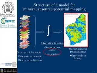
This document explores the utilization of Geographic Information Systems (GIS) for mapping the potential of mineral resources through probabilistic methods. It emphasizes the role of Weights-of-Evidence modeling and logistic regression in estimating the probabilities of various types of mineral deposits. Key formulas like Bayes' Rule and logistics are detailed to demonstrate how uncertainties, including those from missing data, affect mineral resource estimates. An example from the Meguma Terrain illustrates the application of these techniques in real-world scenarios.

E N D
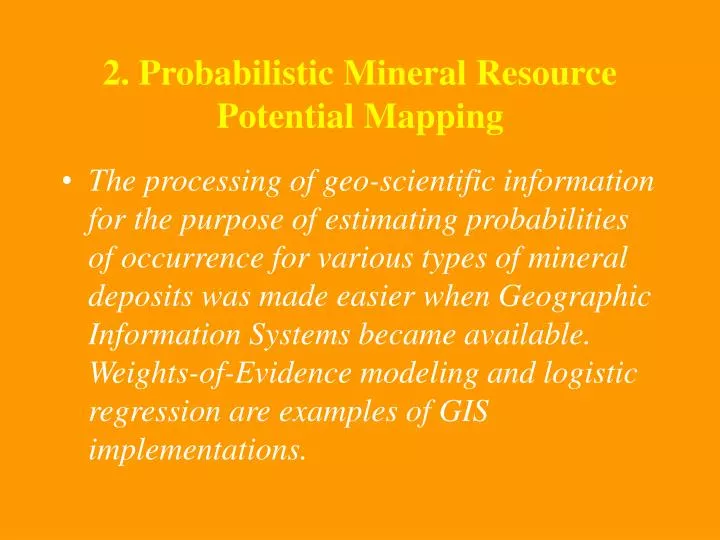
2. Probabilistic Mineral Resource Potential Mapping • The processing of geo-scientific information for the purpose of estimating probabilities of occurrence for various types of mineral deposits was made easier when Geographic Information Systems became available. Weights-of-Evidence modeling and logistic regression are examples of GIS implementations.
BAYES’ RULE P(D on A) = P(D and A)/P(A) P(A on D) = P(A and D)/P(D) P(D on A) = P(A on D) * P(D)/P(A)
ODDS & LOGITS O = P/(1-P); P = O/(1+O); logit = ln O ln O(D on A) = W+(A) + ln O(D) W+(A) = ln {P(A on D)/P(A not on D)}
VARIANCE OF WEIGHT s2 = n-1(A and D) + n-1(A and not D)
Negative Weight & Contrast W-(A) = W+(not A) Contrast: C = W+(A) - W-(A)
PRESENT, ABSENT or MISSING add W+, W- or 0 to prior logit
TWO or MORE LAYERS Add Weight(s) assuming Conditional Independence P(<A and B> on D) = P(A on D) * P(B on D)
UNCERTAINTY DUE TO MISSING DATA P(D) = EX{P(D on X)} = S P(D on Ai) * P(Ai) or S P(D on <Ai and Bk>) * P(<Ai and Bk>) etc.
VARIANCE (MISSING DATA) s2{P(D)} = S {P(D on Ai) - P(D)}2 * P(Ai) or S {P(D on <Ai and Bk>) - P(D)}2 * P(<Ai and Bk>) etc.
TOTAL UNCERTAINTY Var (Posterior Logit) = Var (Prior Logit) + + S Var (Weights) + Var (Missing Data)
Uncertainty inLogits and Probabilities D {Logit (P)} = 1/P(1-P) s(P) ~ P(1-P) s{Logit (P)}
Table 1. Number of gold deposits, area in km2, weights, contrast (C) with standard deviations (s). In total: 68 deposits on 2945 km2
Logistic Regression Logit (i) = b0 + xi1b1 + xi2b2 + … + xim bm
Newton-Raphson Iteration b(t+1) = b(t) + {XTV(t)X)}-1XTr(t), t = 1, 2, … r(t) = y(t) - p(t)