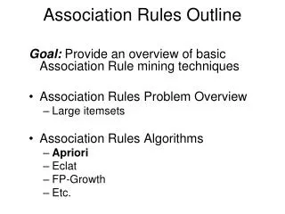
Association Rules Outline
Association Rules Outline. Goal: Provide an overview of basic Association Rule mining techniques Association Rules Problem Overview Large itemsets Association Rules Algorithms Apriori Eclat. Example: Market Basket Data. Items frequently purchased together: Bread PeanutButter Uses:

Association Rules Outline
E N D
Presentation Transcript
Association Rules Outline Goal: Provide an overview of basic Association Rule mining techniques • Association Rules Problem Overview • Large itemsets • Association Rules Algorithms • Apriori • Eclat
Example: Market Basket Data • Items frequently purchased together: Bread PeanutButter • Uses: • Placement • Advertising • Sales • Coupons • Objective: increase sales and reduce costs
Association Rule Definitions • Set of items: I={I1,I2,…,Im} • Transactions: D={t1,t2, …, tn}, tj I • Itemset: {Ii1,Ii2, …, Iik} I • Support of an itemset: Percentage of transactions which contain that itemset. • Large (Frequent) itemset: Itemset whose number of occurrences is above a threshold.
Association Rules Example I = { Beer, Bread, Jelly, Milk, PeanutButter} Support of {Bread,PeanutButter} is 60%
Association Rule Definitions • Association Rule (AR): implication X Y where X,Y I and X Y = ; • Support of AR (s) X Y: Percentage of transactions that contain X Y • Confidence of AR (a) X Y: Ratio of number of transactions that contain X Y to the number that contain X
Association Rule Problem • Given a set of items I={I1,I2,…,Im} and a database of transactions D={t1,t2, …, tn} where ti={Ii1,Ii2, …, Iik} and Iij I, the Association Rule Problem is to identify all association rules X Y with a minimum support and confidence. • Link Analysis • NOTE: Support of X Y is same as support of X Y.
Association Rule Techniques • Find Large Itemsets. • Generate rules from frequent itemsets.
Apriori • Large Itemset Property: Any subset of a large itemset is large. • Contrapositive: If an itemset is not large, none of its supersets are large.
Apriori Ex (cont’d) s=30% a = 50%
Apriori Algorithm • C1 = Itemsets of size one in I; • Determine all large itemsets of size 1, L1; • i = 1; • Repeat • i = i + 1; • Ci = Apriori-Gen(Li-1); • Count Ci to determine Li; • until no more large itemsets found;
Apriori-Gen • Generate candidates of size i+1 from large itemsets of size i. • Approach used: join large itemsets of size i if they agree on i-1 • May also prune candidates who have subsets that are not large.
Apriori Adv/Disadv • Advantages: • Uses large itemset property. • Easily parallelized • Easy to implement. • Disadvantages: • Assumes transaction database is memory resident. • Requires up to m database scans.
Classification based on Association Rules (CBA) • Why? • Can effectively uncover the correlation structure in data • AR are typically quite scalable in practice • Rules are often very intuitive • Hence classifier built on intuitive rules is easier to interpret • When to use? • On large dynamic datasets where class labels are available and the correlation structure is unknown. • Multi-class categorization problems • E.g. Web/Text Categorization, Network Intrusion Detection
Example: Text categorization • Input • <feature vector> <class label(s)> • <feature vector> = w1,…,wN • <class label(s)> = c1,…,cM • Run AR with minsup and minconf • Prune rules of form • w1 w2, [w1,c2] c3 etc. • Keep only rules satisfying the constraing • W C (LHS only composed of w1,…wN and RHS only composed of c1,…cM)
CBA: Text Categorization (cont.) • Order remaining rules • By confidence • 100% • R1: W1 C1 (support 40%) • R2: W4 C2 (support 60%) • 95% • R3: W3 C2 (support 30%) • R4: W5 C4 (support 70%) • And within each confidence level by support • Ordering R2, R1, R4, R3
CBA: contd • Take training data and evaluate the predictive ability of each rule, prune away rules that are subsumed by superior rules • T1: W1 W5 C1,C4 • T2: W2 W4 C2 Note: only subset • T3: W3 W4 C2 of transactions • T4: W5 W8 C4 in training data • T5: W9 C2 • Rule R3 would be pruned in this example if it is always subsumed by Rule R2 • For remaining transactions pick most dominant class as default • T5 is not covered, so C2 is picked in this example
Formal Concepts of Model • Given two rules ri and rj, define: ri rj if The confidence of ri is greater than that of rj, or Their confidences are the same, but the support of ri is greater than that of rj, or Both the confidences and supports are the same, but ri is generated earlier than rj. • Our classifier model is of the following format: <r1, r2, …, rn, default_class>, where ri R, ra rb if b>a • Other models possible • Sort by length of antecedent
Using the CBA model to classify • For a new transaction • W1, W3, W5 • Pick the k-most confident rules that apply (using the precedence ordering established in the baseline model) • The resulting classes are the predictions for this transaction • If k = 1 you would pick C1 • If k = 2 you would pick C1, C2 (multi-class) • Similarly if W9, W10 you would pick C2 (default) • Accuracy measurements as before (Classification Error)
CBA: Procedural Steps • Preprocessing, Training and Testing data split • Compute AR on Training data • Keep only rules of form X C • C is class label itemset and X is feature itemset • Order AR • According to confidence • According to support (at each confidence level) • Prune away rules that lack sufficient predictive ability on Training data (starting top-down) • Rule subsumption • For data that is not predictable pick most dominant class as default class • Test on testing data and report accuracy
Apriori Adv/Disadv • Advantages: • Uses large itemset property. • Easily parallelized • Easy to implement. • Disadvantages: • Assumes transaction database is memory resident. • Requires up to m database scans.
Vertical Layout • Rather than have • Transaction ID – list of items (Transactional) • We have • Item – List of transactions (TID-list) • Now to count itemset AB • Intersect TID-list of itemA with TID-list of itemB • All data for a particular item is available
Eclat Algorithm • Dynamically process each transaction online maintaining 2-itemset counts. • Transform • Partition L2 using 1-item prefix • Equivalence classes - {AB, AC, AD}, {BC, BD}, {CD} • Transform database to vertical form • Asynchronous Phase • For each equivalence class E • Compute frequent (E)
Asynchronous Phase • Compute Frequent (E_k-1) • For all itemsets I1 and I2 in E_k-1 • If (I1 ∩ I2 >= minsup) add I1 and I2 to L_k • Partition L_k into equivalence classes • For each equivalence class E_k in L_k • Compute_frequent (E_k) • Properties of ECLAT • Locality enhancing approach • Easy and efficient to parallelize • Few scans of database (best case 2)
Max-patterns • Frequent pattern {a1, …, a100} (1001) + (1002) + … + (110000) = 2100-1 = 1.27*1030 frequent sub-patterns! • Max-pattern: frequent patterns without proper frequent super pattern • BCDE, ACD are max-patterns • BCD is not a max-pattern Min_sup=2
Frequent Closed Patterns • Conf(acd)=100% record acd only • For frequent itemset X, if there exists no item y s.t. every transaction containing X also contains y, then X is a frequent closed pattern • “acd” is a frequent closed pattern • Concise rep. of freq pats • Reduce # of patterns and rules • N. Pasquier et al. In ICDT’99 Min_sup=2
Mining Various Kinds of Rules or Regularities • Multi-level, quantitative association rules, correlation and causality, ratio rules, sequential patterns, emerging patterns, temporal associations, partial periodicity • Classification, clustering, iceberg cubes, etc.
uniform support reduced support Level 1 min_sup = 5% Milk [support = 10%] Level 1 min_sup = 5% Level 2 min_sup = 5% 2% Milk [support = 6%] Skim Milk [support = 4%] Level 2 min_sup = 3% Multiple-level Association Rules • Items often form hierarchy • Flexible support settings: Items at the lower level are expected to have lower support. • Transaction database can be encoded based on dimensions and levels • explore shared multi-level mining
ML/MD Associations with Flexible Support Constraints • Why flexible support constraints? • Real life occurrence frequencies vary greatly • Diamond, watch, pens in a shopping basket • Uniform support may not be an interesting model • A flexible model • The lower-level, the more dimension combination, and the long pattern length, usually the smaller support • General rules should be easy to specify and understand • Special items and special group of items may be specified individually and have higher priority
Multi-dimensional Association • Single-dimensional rules: buys(X, “milk”) buys(X, “bread”) • Multi-dimensional rules: 2 dimensions or predicates • Inter-dimension assoc. rules (no repeated predicates) age(X,”19-25”) occupation(X,“student”) buys(X,“coke”) • hybrid-dimension assoc. rules (repeated predicates) age(X,”19-25”) buys(X, “popcorn”) buys(X, “coke”)
Multi-level Association: Redundancy Filtering • Some rules may be redundant due to “ancestor” relationships between items. • Example • milk wheat bread [support = 8%, confidence = 70%] • 2% milk wheat bread [support = 2%, confidence = 72%] • We say the first rule is an ancestor of the second rule. • A rule is redundant if its support is close to the “expected” value, based on the rule’s ancestor.
Multi-Level Mining: Progressive Deepening • A top-down, progressive deepening approach: • First mine high-level frequent items: milk (15%), bread (10%) • Then mine their lower-level “weaker” frequent itemsets: 2% milk (5%), wheat bread (4%) • Different min_support threshold across multi-levels lead to different algorithms: • If adopting the same min_support across multi-levels then toss t if any of t’s ancestors is infrequent. • If adopting reduced min_support at lower levels then examine only those descendents whose ancestor’s support is frequent/non-negligible.
Interestingness Measure: Correlations (Lift) • play basketball eat cereal [40%, 66.7%] is misleading • The overall percentage of students eating cereal is 75% which is higher than 66.7%. • play basketball not eat cereal [20%, 33.3%] is more accurate, although with lower support and confidence • Measure of dependent/correlated events: lift
Constraint-based Data Mining • Finding all the patterns in a database autonomously? — unrealistic! • The patterns could be too many but not focused! • Data mining should be an interactive process • User directs what to be mined using a data mining query language (or a graphical user interface) • Constraint-based mining • User flexibility: provides constraints on what to be mined • System optimization: explores such constraints for efficient mining—constraint-based mining
Constrained Frequent Pattern Mining: A Mining Query Optimization Problem • Given a frequent pattern mining query with a set of constraints C, the algorithm should be • sound: it only finds frequent sets that satisfy the given constraints C • complete: all frequent sets satisfying the given constraints C are found • A naïve solution • First find all frequent sets, and then test them for constraint satisfaction • More efficient approaches: • Analyze the properties of constraints comprehensively • Push them as deeply as possible inside the frequent pattern computation.
Anti-Monotonicity in Constraint-Based Mining TDB (min_sup=2) • Anti-monotonicity • When an intemset S violates the constraint, so does any of its superset • sum(S.Price) v is anti-monotone • sum(S.Price) v is not anti-monotone • Example. C: range(S.profit) 15 is anti-monotone • Itemset ab violates C • So does every superset of ab
Monotonicity in Constraint-Based Mining TDB (min_sup=2) • Monotonicity • When an intemset S satisfies the constraint, so does any of its superset • sum(S.Price) v is monotone • min(S.Price) v is monotone • Example. C: range(S.profit) 15 • Itemset ab satisfies C • So does every superset of ab
Succinctness • Succinctness: • Given A1, the set of items satisfying a succinctness constraint C, then any set S satisfying C is based on A1, i.e., S contains a subset belonging to A1 • Idea: Without looking at the transaction database, whether an itemset S satisfies constraint C can be determined based on the selection of items • min(S.Price) v is succinct • sum(S.Price) v is not succinct • Optimization: If C is succinct, C is pre-counting pushable
The Apriori Algorithm — Example Database D L1 C1 Scan D C2 C2 L2 Scan D L3 C3 Scan D
Naïve Algorithm: Apriori + Constraint Database D L1 C1 Scan D C2 C2 L2 Scan D L3 C3 Constraint: Sum{S.price < 5} Scan D
Pushing the constraint deep into the process Database D L1 C1 Scan D C2 C2 L2 Scan D L3 C3 Constraint: Sum{S.price < 5} Scan D
Push a Succinct Constraint Deep Database D L1 C1 Scan D C2 C2 L2 Scan D L3 C3 Constraint: min{S.price <= 1 } Scan D