Download
1 / 27
270 likes | 491 Vues
Tails of Copulas. Gary G Venter. Correlation Issues. Correlation is stronger for large events Can model by copula methods Quantifying correlation Degree of correlation Part of spectrum correlated. Modeling via Copulas. Correlate on probabilities

E N D
Tails of Copulas Gary G Venter
Correlation Issues • Correlation is stronger for large events • Can model by copula methods • Quantifying correlation • Degree of correlation • Part of spectrum correlated
Modeling via Copulas • Correlate on probabilities • Inverse map probabilities to correlate losses • Can specify where correlation takes place in the probability range • Conditional distribution easily expressed • Simulation readily available
What is a copula? • A way of specifying joint distributions • A way to specify what parts of the marginal distributions are correlated • Works by correlating the probabilities, then applying inverse distributions to get the correlated marginal distributions • Formally they are joint distributions of unit uniform variates, as probabilities are uniform on [0,1]
Formal Rules • F(x,y) = C(FX(x),FY(y)) • Joint distribution is copula evaluated at the marginal distributions • Expresses joint distribution as inter-dependency applied to the individual distributions • C(u,v) = F(FX-1(u),FY-1(v)) • u and v are unit uniforms, F maps R2 to [0,1] • FY|X(y) = C1(FX(x),FY(y)) • Derivative of the copula is the conditional distribution • E.g., C(u,v) = uv, C1(u,v) = v = Pr(V<v|U=u) • So independence copula
Correlation • Kendall tau and rank correlation depend only on copula, not marginals • Not true for linear correlation rho • Tau may be defined as: –1+4E[C(u,v)]
Example C(u,v) Functions • Frank: -a-1ln[1 + gugv/g1], with gz = e-az – 1 • t(a) = 1 – 4/a + 4/a20at/(et-1) dt • Gumbel: exp{- [(- ln u)a + (- ln v)a]1/a}, a 1 • t(a) = 1 – 1/a • HRT: u + v – 1+[(1 – u)-1/a + (1 – v)-1/a – 1]-a • t(a) = 1/(2a + 1) • Normal: C(u,v) = B(p(u),p(v);a) i.e., bivariate normal applied to normal percentiles of u and v, correlation a • t(a) = 2arcsin(a)/p
Copulas Differ in Tail EffectsLight Tailed Copulas Joint Lognormal
Copulas Differ in Tail EffectsHeavy Tailed Copulas Joint Lognormal
Partial Perfect Correlation Copulas of Kreps • Each simulated probability pair is either identical or independent depending on symmetric function h(u,v), often =h(u)h(v) • h(u,v) –> [0,1], e.g., h(u,v) = (uv)3/5 • Draw u,v,w from [0,1] • If h(u,v)>w, drop v and set v=u • Simulate from u and v, which might be u
Partial Perfect Copula Formulas • For case h(u,v)=h(u)h(v) • H’(u)=h(u) • C(u,v) = uv – H(u)H(v) + H(1)H(min(u,v)) • C1(u,v) = v – h(u)H(v) + H(1)h(u)(v>u)
Tau’s • h(u)=ua, t(a)= (a+1)-4/3 +8/[(a+1)(a+2)2(a+3)] • h(u)=(u>k), t(k) = (1 – k)4 • h(u)=h0.5, t(h) = (h2+2h)/3 • h(u)= h0.5ua(u>k), t(h,a,k) = h2(1-ka+1)4(a+1)-4/3 +8h[(a+2)2(1-ka+3)(1-ka+1)–(a+1)(a+3)(1-ka+2)2]/d where d = (a+1)(a+2)2(a+3)
Quantifying Tail Concentration • L(z) = Pr(U<z|V<z) • R(z) = Pr(U>z|V>z) • L(z) = C(z,z)/z • R(z) = [1 – 2z +C(z,z)]/(1 – z) • L(1) = 1 = R(0) • Action is in R(z) near 1 and L(z) near 0 • lim R(z), z->1 is R, and lim L(z), z->0 is L
Example: ISO Loss and LAE • Freez and Valdez find Gumbel fits best, but only assume Paretos • Klugman and Parsa assume Frank, but find better fitting distributions than Pareto All moments less than tail parameter converge
Can Try Joint Burr, from HRT • F(x,y) = 1–(1+(x/b)p)-a –(1+(y/d)q)-a +[1+(x/b)p +(y/d)q]-a • E.g. F(x,y)=1–[1+x/14150]-1.11–[1+(y/6450)1.5]-1.11 +[1+x/14150 +(y/6450)1.5]-1.11 • Given loss x, conditional distribution is Burr: • FY|X(y|x) = 1–[1+(y/dx)1.5]–2.11 • with dx = 6450 +11x 2/3
L and R Functions, Tau = .45 • R looks about .25, which is >0, <tau, so none of our copulas match
Modified Tail Concentration Functions • Both MLE and R function show that HRT fits best
Conclusions • Copulas allow correlation of different parts of distributions • Tail functions help describe and fit