Download
1 / 20
200 likes | 305 Vues
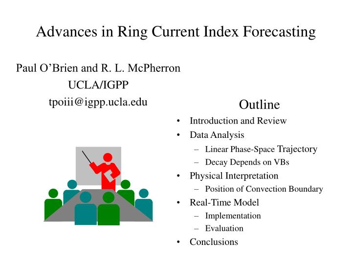
Outline Introduction and Review Data Analysis Linear Phase-Space Trajectory Decay Depends on VBs Physical Interpretation Position of Convection Boundary Real-Time Model Implementation Evaluation Conclusions. Advances in Ring Current Index Forecasting. Paul O’Brien and R. L. McPherron

E N D
Outline Introduction and Review Data Analysis Linear Phase-Space Trajectory Decay Depends on VBs Physical Interpretation Position of Convection Boundary Real-Time Model Implementation Evaluation Conclusions Advances in Ring Current Index Forecasting Paul O’Brien and R. L. McPherron UCLA/IGPP tpoiii@igpp.ucla.edu
Meet the Ring Current March 97 Magnetic Storm Recovery 100 0 • During a magnetic storm, Southward IMF reconnects at the dayside magnetopause • Magnetospheric convection is enhanced & hot particles are injected from the ionosphere • Trapped radiation between L ~2-10 sets up the ring current, which can take several days to decay away • We measure the magnetic field from this current as Dst Dst (nT) -100 -200 Injection -300 91 92 93 94 95 96 97 98 99 Pressure Effect 10 VBs (mV/m) 5 0 91 92 93 94 95 96 97 98 99 60 40 Psw (nPa) 20 0 91 92 93 94 95 96 97 98 99 Day of Year
DDst Distribution (Main Phase) No Data DDst Q - Dst/t Median Trajectory No Data
The Trapping-Loss Connection t Decreases • The convection electric field shrinks the convection pattern • The Ring Current is confined to the region of higher nH, which results in shorter t • The convection electric field is related to VBs Larger VBs
Decay Time (t) 20 18 t from Phase-Space Slope Points Used in Fit 16 t = 2.40e9.74/(4.69+VBs) 14 12 t (hours) 10 8 6 4 2 0 2 4 6 8 10 12 VBs (mV/m) Fit of t vs VBs • The derived functional form can fit the data with physically reasonable parameters • Our 4.69 is slightly larger than 1.1 from Reiff et al. ?
t for various ranges of Dst (with specification of VBs) t for various ranges of Dst (without specification of VBs) 20 20 VBs = 0 All VBs 18 18 VBs = 0 VBs = 2 VBs = 4 16 16 14 14 VBs = 2 t (hours) t (hours) 12 12 10 10 VBs = 4 8 8 6 6 4 4 -200 -150 -100 -50 0 -200 -150 -100 -50 0 Dst Range (nT) Dst Range (nT) How to Calculate the Wrong Decay Rate • Using a least-squares fit of DDst to Dst we can estimate t • If we do this without first binning in VBs, we observe that t depends on Dst • If we first bin in VBs, we observe that t depends much more strongly on VBs • A weak correlation between VBs and Dst causes the apparent t-Dst dependence
Dst Comparison for storm 1980-285 Dst Comparison for storm 1982-061 20 50 0 0 -20 -50 -40 Dst (nT) Dst (nT) -100 Dst -60 Dst Model (1hr step) -150 Model (multi-step) Model (1hr step) -80 Model (multi-step) VBs -200 VBs -100 -120 -250 0 20 40 60 80 100 120 140 160 180 0 50 100 150 15 6 5 10 4 VBs mV/m VBs mV/m 3 5 2 Ec = 0.49 mV/m Ec = 0.49 mV/m 1 0 0 0 20 40 60 80 100 120 140 160 180 0 50 100 150 Epoch Hours Epoch Hours Small & Big Storms
More errors are associated with large VBs than with large Dst Dst Transitions for 1982-061 Dst Transitions for 1980-285 20 50 0 0 -20 -50 -40 Error Error Dst (nT) Dst (nT) -100 VBs > Ec VBs > Ec -60 VBs > 5 VBs > 5 -150 -80 -200 -100 -120 -250 -50 -40 -30 -20 -10 0 10 20 30 40 50 -50 -40 -30 -20 -10 0 10 20 30 40 50 Error: Model-Dst (nT) Error: Model-Dst (nT) Small & Big Storm Errors
ACE/Kyoto System • The Kyoto World Data Center provides provisional Dst estimate about 12-24 hours behind real-time • The Space Environment Center provides real-time measurements of the solar wind from the ACE spacecraft • We use our model to integrate from the last Kyoto data to the arrival of the last ACE measurement • This usually amounts to a forecast of 45+ minutes
50 50 0 0 -50 -50 -100 Kyoto Dst nT nT AK2 -150 -100 AK1 UCB -200 ACE Gap -150 -250 -200 -300 308 310 312 314 316 318 320 322 324 326 266 267 268 269 270 271 272 273 274 275 276 UT Decimal Day (1998) UT Decimal Day (1998) Comparisons to Other Models ACE Gap AK2 is the new model, Kyoto is the target, AK1 is a strictly Burton model, and UCB has slightly modified injection and decay. AK2 has a skill score of 30% relative to AK1 and 40% relative to UCB for 6 months of simulated real-time data availability. These numbers are even better if only active times are used.
Error Distributions For 3 Real-Time Models 0.16 UCB Bin Size: 5 nT AK1 0.14 AK2 0.12 0.1 Fraction of All Points 0.08 0.06 0.04 0.02 0 -50 -40 -30 -20 -10 0 10 20 30 40 50 Error (nT) Details of Model Errors in Simulated Real-Time Mode ACE availability was 91% (by hour) in 232 days Predicting large Dst is difficult, but larger errors may be tolerated in certain applications
Real-Time Dst On-Line • With real-time Solar wind data from ACE and near real-time magnetic measurements from Kyoto, we can provide a real-time forecast of Dst • We publish our Dst forecast on the Web every 30 minutes
Summary • Dst follows a first order equation: • dDst/dt = Q(VBs) - Dst/t(VBs) • Injection and decay depend on VBs • Dst dependence is very weak or absent • We have suggested a mechanism for the decay dependence on VBs • Convection is brought closer to the exosphere by the cross-tail electric field • The model performs well in real-time relative to two other models • Poorest performance for large VBs
Looking Forward • The USGS now provides measurements of H from SJG, HON, and GUA only 15 minutes behind real-time • If we can convert H into DH in real-time, we can use a 3-station provisional Dst to start our model, and only have to integrate about an hour • We have built Neural Networks which can provide Dst from 1, 2 or 3 DH values and UT local time • Shortening our integration period could greatly reduce the error in our forecast
Motion of Median Trajectory VBs = 0 VBs = 1 mV/m VBs = 2 mV/m VBs = 3 mV/m VBs = 4 mV/m VBs = 5 mV/m As VBs is increased, distributions slide left and tilt, but linear behavior is maintained.
Speculation on t(VBs) The charge-exchange lifetimes are a function of L because the exosphere density drops off with altitude t is an effective charge-exchange lifetime for the whole ring current. t should therefore reflect the charge-exchange lifetime at the trapping boundary • A cross-tail electric field E0 moves the stagnation point for hot plasma closer to the Earth. This is the trapping boundary (p is the shielding parameter) • Reiff et al. 1981 showed that VBs controlled the polar-cap potential drop which is proportional to the cross-tail electric field
Injection (Q) vs VBs 10 0 -10 -20 -30 Injection (Q) (nT/h) -40 -50 Offsets in Phase Space -60 Points Used in Fit Ec = 0.49 Q = (-4.4)(VBs-0.49) -70 -80 0 2 4 6 8 10 12 VBs (mV/m) Q is nearly linear in VBs • The Q-VBs relationship is linear, with a cutoff below Ec • This is essentially the result from Burton et al. (1975)
VBs = 0 VBs = 1 VBs = 2 VBs = 3 NN Dst VBs = 4 Stat Dst VBs = 5 Neural Network Verification DDst = NN(Dst,VBs,…) Neural Network Phase Space 0 • A neural network provides good agreement in phase space • The curvature outside the HTD area may not be real High Training Density -50 Dst -100 -150 -25 -20 -15 -10 -5 0 5 10 15 DDst
Phase Space Trajectories Simple Decay Oscillatory Decay Dst(t) Dst(t) Variable Decay Dst(t+dt)-Dst(t) Dst(t+dt)-Dst(t) Dst(t) Dst(t+dt)-Dst(t)
(Phase-Space Offset) - Q vs D[P1/2] 6 4 2 0 -2 (PS Offset) -Q (nT/h) -4 (PS Offset) - Q -6 Best Fit ~ (7.26) D[P1/2] -8 -10 -12 -0.6 -0.4 -0.2 0 0.2 0.4 0.6 0.8 D[P1/2] (nPa1/2/h) Calculation of Pressure Correction • So far, we have assumed that the pressure correction was not important.This is true because: But now we would like to determine the coefficients b and c. We can determine b by binning in D[P1/2] and removing Q(VBs) We can determine c such that Dst* decays to zero when VBs = 0