Schema Tuning
Schema Tuning. Outline. Index Utilization Heap Files Definition: Clustered/Non clustered, Dense/Sparse Access method: Types of queries Constraints and Indexes Locking Index Data Structures B+-Tree / Hash LSM Tree / Fractal tree Implementation in DBMS Index Tuning


Schema Tuning
E N D
Presentation Transcript
Schema Tuning @ Dennis Shasha and Philippe Bonnet, 2013
Outline • Index Utilization • Heap Files • Definition: Clustered/Non clustered, Dense/Sparse • Access method: Types of queries • Constraints and Indexes • Locking • Index Data Structures • B+-Tree / Hash • LSM Tree / Fractal tree • Implementation in DBMS • Index Tuning • Index data structure • Search key • Size of key • Clustered/Non-clustered/No index • Covering
Database Schema • A relation schema is a relation name and a set of attributes R(a int, b varchar[20]); • A relation instance for R is a set of records over the attributes in the schema for R.
Space Schema 2 saves space Information preservation Some supplier addresses might get lost with schema 1. Performance trade-off Frequent access to address of supplier given an ordered part, then schema 1 is good. Many new orders, schema 1 is not good. Some Schema are better than others • Schema1: OnOrder1(supplier_id, part_id, quantity, supplier_address) • Schema 2: OnOrder2(supplier_id, part_id, quantity); Supplier(supplier_id, supplier_address);
Functional Dependencies • X is a set of attributes of relation R, and A is a single attribute of R. • X determines A (the functional dependency X-> A holds for R) iff: • For any relation instance I of R, whenever there are two records r and r’ in I with the same X values, they have the same A value as well. • OnOrder1(supplier_id, part_id, quantity, supplier_address) • supplier_id ->supplier_address is an interesting functional dependency
Key of a Relation • Attributes X from R constitute a key of R if X determines every attribute in R and no proper subset of X determines an attribute in R. • OnOrder1(supplier_id, part_id, quantity, supplier_address) • supplier_id, part_id is not a key • Supplier(supplier_id, supplier_address); • Supplier_id is a key
Normalization • A relation is normalized if every interesting functional dependency X-> A involving attributes in R has the property that X is a key of R • OnOrder1 is not normalized • OnOrder2 and Supplier are normalized • Here normalized, refers to BCNF (Boyce-Codd Normal Form)
Example #1 • Suppose that a bank associates each customer with his or her home branch. Each branch is in a specific legal jurisdiction. • Is the relation R(customer, branch, jurisdiction) normalized?
Example #1 • What are the functional dependencies? • Customer -> branch • Branch -> jurisdiction • Customer -> jurisdiction • Customer is the key, but a functional dependency exists where customer is not involved. • R is not normalized.
Example #2 • Suppose that a doctor can work in several hospitals and receives a salary from each one. Is R(doctor, hospital, salary) normalized?
Example #2 • What are the functional dependencies? • doctor, hospital -> salary • The key is doctor, hospital • The relation is normalized.
Example #3 • Same relation R(doctor, hospital, salary) and we add the attribute primary_home_address. Each doctor has a primary home address and several doctors can have the same primary home address. Is R(doctor, hospital, salary, primary_home_address) normalized?
Example #3 • What are the functional dependencies? • doctor, hospital -> salary • Doctor -> primary_home_address • doctor, hospital -> primary_home_address • The key is no longer doctor, hospital because doctor (a subset) determines one attribute. • A normalized decomposition would be: • R1(doctor, hospital, salary) • R2(doctor, primary_home_address)
Practical Schema Design • Identify entities in the application (e.g., doctors, hospitals, suppliers). • Each entity has attributes (an hospital has an address, a juridiction, …). • There are two constraints on attributes: • An attribute cannot have attribute of its own (1FN) • The entity associated with an attribute must functionally determine that attribute.
Practical Schema Design • Each entity becomes a relation • To those relations, add relations that reflect relationships between entities. • Worksin (doctor_ID, hospital_ID) • Identify the functional dependencies among all attributes and check that the schema is normalized: • If functional dependency AB →C holds, then ABC should be part of the same relation.
Compression • Index level • Key compression • Tablespace level • All blocks in a tablespace are compressed • Blocks are compressed/uncompressed as they are transferred between RAM and secondary storage. • Row level • All rows in a table are compressed
Compression Methods • Lossless methods • Exploits redundancy to represent data concisely • Differential encoding (difference of adjacent values in the same column or same tuple) • Offset encoding (offset to a base value) • Prefix compression (index keys) • Null suppression (omit lead zero bytes or spaces) • Non adaptive dictionary encoding • Adaptive dictionary encoding (LZ77) • Huffman encoding (assign fewer bits to represent frequent characters) • Arithmetic encoding (interval representation of a string according to probability of each character)
Compression Trade-offs • CPU / IO • Compression/decompression is CPU intensive, reduces IO cost • Fewer IOs to transfer data from secondary storage to RAM • Overall DB footprint is smaller • Trade-off accounted for • During calibration • At run time: alter table to activate/deactivate compression. • DBMS/SSD • Some SSD support compression. This should be turned off. Compression should be managed at DBMS level.
Tuning Normalization • A single normalized relation XYZ is better than two normalized relations XY and XZ if the single relation design allows queries to access X, Y and Z together without requiring a join. • The two-relation design is better iff: • Users access tend to partition between the two sets Y and Z most of the time • Attributes Y or Z have large values
Vertical Partitioning • Three attributes: account_ID, balance, address. • Functional dependencies: • account_ID -> balance • account_ID -> address • Two normalized schema design: • (account_ID, balance, address) or • (account_ID, balance) • (account_ID, address) • Which design is better?
The second schema might be better because the relation (account_ID, balance) can be made smaller: More account_ID, balance pairs fit in memory, thus increasing the hit ratio A scan performs better because there are fewer pages. Vertical Partitioning • Which design is better depends on the query pattern: • The application that sends a monthly statement is the principal user of the address of the owner of an account • The balance is updated or examined several times a day.
Vertical Antipartitioning • Brokers base their bond-buying decisions on the price trends of those bonds. The database holds the closing price for the last 3000 trading days, however the 10 most recent trading days are especially important. • (bond_id, issue_date, maturity, …)(bond_id, date, price) Vs. • (bond_id, issue_date, maturity, today_price, …10dayago_price)(bond_id, date, price)