Download
1 / 28
280 likes | 378 Vues
Learn about quantum states in different barriers, including infinite well and central barriers, and how they affect particle behavior. Understand energy level splitting in chemistry and the concept of quantum mechanical tunneling.

E N D
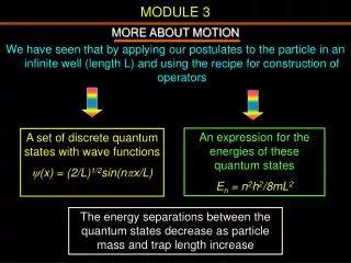
MODULE 3 MORE ABOUT MOTION We have seen that by applying our postulates to the particle in an infinite well (length L) and using the recipe for construction of operators An expression for the energies of these quantum states En = n2h2/8mL2 A set of discrete quantum states with wave functions y(x) = (2/L)1/2sin(npx/L) The energy separations between the quantum states decrease as particle mass and trap length increase
MODULE 3 With particles of macroscopic mass, the quantum states still exist but the energy separation becomes far too small to detect. The same thing occurs as the enclosure becomes larger. With an enclosure of infinite length the zero point energy approaches zero and the energy levels coalesce, yielding the free particle situation. Thus the quantum description of matter applies to all sizes of particle and enclosure--it is simply that the effects are discernable only with submicroscopic systems.
I II III V(x) = U V(x) = U V(x) = 0 MODULE 3 What if the constraining barriers to the particle are less than infinite? Consider a 1-dimensional well with barriers of height V(x) = U, where U <<∞ Regions I and III are identical (V(x) = U)
MODULE 3 Two situations to consider: E<UandE>U (i) E < U A classical particle with E < U would never escape the well. Its kinetic energy (= E, since V = 0) would not be enough to allow it to jump over the barrier. Let us see what the quantum theory approach tells us. In regions I and III (identical, V = U) and V = U
MODULE 3 A well-behaved wavefunction must not go to infinity both these are declining exponentials because x is negative in region I and positive in region III yI,yIII tend to 0 as x tends to so the well-behavedness holds
MODULE 3 To find the form of the wavefunction in region II is complicated so we guess that the form will be oscillatory, in the same way as are the solutions for the infinitely high walls. The difference, however is in the boundary conditions. Now yI and yIII are non-zero where they meet the wall and wavefunctions and their derivatives must be continuous. So yI and yIII must both join seamlessly to yII at the wall.
n = 1 n = 2 MODULE 3 These boundary conditions lead to a set of discrete states, denoted by integral quantum numbers (n=1, 2, 3, ...). The wavefunctions extend beyond the walls of the trap into regions that are forbidden to a classical particle The wavelength is longer than for the corresponding state in the infinite wall and therefore the energy is lower (less curvature). since E<U therefore E-U = kinetic energy < 0 i.e. the kinetic energy of the particle in I and III is negative.
MODULE 3 the probability density is given by y2and there is a non-zero probability of the particle being found outside the confines. as E approaches U (recall E < U) this probability will increase. Also, as U goes to infinity the amplitudes of the wavefunctions outside region II approach zero, and in the limit the wavefunction becomes identical with that of the infinite wall case. Moreover the exponential amplitudes are proportional to m, which tells us that the lighter the particle, the more barrier penetration we shall find.
MODULE 3 If the barrier is sufficiently narrow, the wavefunction will not have fallen to zero at the outer edge. In this case the wavefunction will propagate as a free particle outside the walls and the oscillations will continue to infinity unless some other potential energy barriers get in the way. This is called quantum mechanical tunneling. It is an extreme example of barrier penetration and is purely QM
MODULE 3 Finite central barrier in infinite well Wavefunctions penetrate barrier and overlap and interact inside it Symmetric overlap causes wavelength to be longer (lower energy) Antisymmetric overlap creates higher energy states
MODULE 3 Energy level splitting occurs in many situations in chemistry. We see later that overlap of a pair of atomic orbitals leads to a pair of molecular orbitals, one of lower energy (bonding) and one of higher energy than the initial AOs. Inversion of pyramidal NH3 causes vibrational level splitting The interaction (symmetric and antisymmetric) of the pair of configurations separated by the higher energy planar configuration leads to energy level splittings near 0.02 zJ (DE1) in the microwave spectral region.
MODULE 3 In the situation where E>U, the (U-E)1/2 terms are imaginary. the complete wave function continues to infinity in an uninterrupted way, in the manner of a classical particle. In the vicinity of the two wells, where V = 0, all E is kinetic energy In the region of space where V = U (the barrier) only part of E is kinetic (remembering E is independent of x) and we anticipate that the wave function will have a lower curvature than elsewhere.
MODULE 3 Simple Harmonic Motion (SHM) A special case of linear motion. In the macro-world SHM is exhibited by pendula and masses attached to springs. These have an equilibrium (rest) position where no motion occurs. When a force displaces the pendulum, e.g., from its equilibrium a restoring force (F(x)) proportional to the extent of the displacement is generated.
MODULE 3 The PE curve for a harmonic oscillator V = kx2/2
MODULE 3 Application of Newton's second law gives This is an eigenvalue equation and a solution is where w = (k/m)1/2 and L is the maximum displacement. Thus the displacement is a harmonic function in time.
MODULE 3 The quantum version SHM is a good model for the stretching and compressing of the chemical bond, viz., bond vibrational motion. A bond undergoes continuous compression and extension. The two atoms move along the bond axis in a similar way to two masses connected by a spring As always, the procedure begins with setting up the Schrödinger equation
MODULE 3 where the kx2/2 is the operator for the potential energy. Now we have an eigenvalue equation in which the potential energy term is not zero. This makes for a major complication in solving. We assume the math can be done and we quote the solutions.
MODULE 3 The wave function solution is a set of discrete functions They are the products of a Gaussian function and a Hermite polynomial. The Hermite functions form a set, each depending on an integer Thus N is a normalizing factor, Hn(y) is the nth Hermite polynomial, and y is given by
n Hn(y)(y) 0 0 11 1 1 1 2y 2y 2 2 4y2-2 4y2-2 3 3 8y3-12y 8y3-12y 4 16y4-48y2+12 16y4-24y2+12 MODULE 3 n arises out of the polynomials. It is a quantum number and can take values n = 0, 1, 2, 3, … The first five Hermite polynomials are
MODULE 3 The first five wavefunctions
MODULE 3 The first and second quantum states of the harmonic oscillator
MODULE 3 The first seven wavefunctions and their probability distributions
MODULE 3 The energy eigenvalues depend on n with n the classical frequency of the harmonic motion and equal to w /2p [recall w =(k/m)1/2], then: When n = 0, E0 = hn /2. This is the zero point energy of the quantum harmonic oscillator The energy levels spacing is constant and equal to hn Real chemical bonds depart from simple harmonic behavior at higher values of n.
MODULE 3 Angular Motion Motion in a circle and motion on a sphere. Consider three kinds of constrained angular motion: • a particle moving in a circular trajectory about a central point. (a mass on a string, or the rotating motion of a CD). • a particle on the surface of a sphere, or in a thin spherical shell. • a particle confined by a centro-symmetric force field.
MODULE 3 A particle on a string in a circular trajectory about a central point No potential barriers during the cycling motion (Vf = 0). To find the energy of the particle due to its motion we use the Schrödinger equation and define the hamiltonian I isthe moment of inertia and analogous to mass in linear motion. I = mr2
MODULE 3 This is an eigenvalue equation and a general solution is With A and B constants The function must be continuous and single valued. As it completes a cycle it must have the same value as at the same point on the previous cycle. If not it will be annihilated by destructive interference. These are the cyclical boundary conditions.
MODULE 3 That is then This equality is satisfied when This is true for integral values of ml [note ] The wavefunctions are limited to values of ml = 0, ±1, ±2… and the corresponding quantized energies are given by As before, boundary conditions leads to quantization. other kinds of angular motion will be considered later.