Structural Equation Modeling
Structural Equation Modeling. Mgmt 291 Lecture 2 – Path Analysis Oct. 5, 2009. Regression Modeling. Y i = β 0 + β 1 X 1i + β 2 X 2i + β 3 X 3i + ε i Formulation of the research question in terms of independent Xs and dependent variable Y To explain (or predict) Y by Xs (one equation)

Structural Equation Modeling
E N D
Presentation Transcript
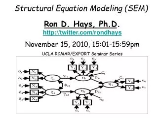
Structural Equation Modeling Mgmt 291 Lecture 2 – Path Analysis Oct. 5, 2009
Regression Modeling • Yi=β0+β1 X1i+β2 X2i + β3 X3i + εi • Formulation of the research question in terms of independent Xs and dependent variable Y • To explain (or predict) Y by Xs (one equation) • Explain the variance of Y • Assumptions: measured without errors, linear, … X1 X1 Y ε X2 X3
In the real world • No clear differentiation between independent variables and dependent variables • How the Xs relate to each other may be important to our research • Not all Xs affect Y directly • Variables may be measured with error
Need to Move from Regression to SEM X1 X1 Y ε X2 X2 X3 Y X1 X3
(1) Selecting SEM Models to Fit Your Data • # of models = 4 n!/2!(n-2)!
(2) Estimating the Coefficients of SEM Model y = a1 + b1 * x + v z = a2 + b2 * y + u u v y z x
FOUR Elements of a Method • 1) Equation (model representation and model types) • 2) Estimation (identification issue and estimation options) • 3) Errors (between data and assumptions) and Evaluation of SEM Models (Fit Indexes) • 4) Explanation of the Results • In these four areas, methods diff from each other.
4 Elements of Regression • 1) Equation - Yi=β0+β1 X1i+β2 X2i + β3 X3i + εi • 2) Estimation – OLS • 3) Errors (Assumptions and Diagnostics) and Evaluation (R2) • 4) Using Bi, t statistics for results Explanation
Part 1: Equations and More -- The Representation of Path Models 3 ways: diagram, equation, table (matrix)
D2 Diagram Rep of path Models Y2 A picture is worth a thousand words X1 X1 Y X1 X2 Y1 Y X2 X2 X3 X4 D1 X3
Equation Rep of Path Models • SEM • Y2i=β0+β1 Y1i+β2 X1i + εi • Y1i=Ø 0+ Ø1 X1i+ Ø 2 X2i + Ø 3 X3i + ε1i • X3i= C0+ C 2 X2i + C 3 X4i + ε2i • Regression • Yi=β0+β1 X1i+β2 X2i + β3 X3i + εi
Table Rep of Path Models • Called as “system matrix”
Example - Diagram • Kline 2005, p67 Fitness Exercise Illness Hardy Stress
Example - equations • Fitness = β0 + β1Exercise + β2Hardiness • Stress = Ø 0 + Ø 1Exercise + Ø 2Hardiness + Ø 3Fitness • Illness = C0 + C1Exercise + C2Hardiness + C3Fitness + C4Stress
Building Blocks of Path Model • 1) Variables – exogenous, endogenous • 2) Relationships – direct, indirect, reciprocal, • 3) Residual – disturbance and (measurement errors) • Similar to regression
Model Complexity 1 • 4 X 3 X 2 X 1 = 24 X1 X2 X3 X4 X1 x1 X2 X4 x4 x2 X3 x3
Model Complexity 2 • Number of observations • = v(v+1) / 2 • Number of model parameters • <= number of observations • # parameters = p + e + d • (p - # paths, e - #obs for exogenous, d - #obs for disturbance) X1 X2 X4 X3
Two Types of Path Models • Recursive • 1) disturbances uncorrelated • 2) no feedback loops • Non-recursive • 1) have feedback loops • 2)or have correlated disturbances
Examples of Recursive Models D1 X1 Y1 D2 X2 X1 Y2 Y1 D1 D2 X2 Y2
Examples of Non-Recursive Models D1 X1 Y1 D2 X2 Y2
Part 2: Estimation Methods for Path Models Identification Issue and Estimation Options
The Identification Issue • whether or not theoretically identifiable • (whether or not the model parameters can be represented by observations – covariances) • Or whether a set of equations can be solved. • Diff Σ (yi – b0 – b1* xi)2 against b0 and b1, then solve two equations to get b0 and b1 for simple regression • similar for SEM (see Duncan’s book)
Examples • Under-identified • x+y = 6 • Just-identified • x+y=6 • 2x+y=10 • Over-identified • x+y=6 • 2x+y=10 • 3x+y=12
The Order Condition • Number of excluded variables >= • (number of endogenous variables – 1) • For each endogenous variable (Kline p306-307) D1 X1 Y1 D2 X2 Y2
The Rank Condition • Use the system matrix • rank >= #endogenous vars - 1 D1 y1 x1 x2 y2 D2 y3 x3 D3
Estimation Options • OLS • ML • OLS and ML produces the identical results for just-identified recursive models, and similar results for over-identified models
About ML • Maximum Likelihood Estimation • Simultaneous • Iterative • (starting values) • Most common used (default method in LISREL and many other programs)
Using OLS for Path Analysis D1 • Ok for recursive models • Not for non-recursive (violate the assumption that residuals uncorrelated with ind vars) X1 Y1 D2 X2 Y2
The Fit Indexes • Chi squares – most common used • d.f. = # obs - # parameters • RMR (mean squared residual) • RMSEA (root mean squared error of approximation) • GFI & AGFT (0 ~ 1) • (Similar to R2 and adjusted R2)
More about Fit indexes • Dozens available • LISREL prints 15 • ChiSquares/df < 3 • GFI > .90 • Inspect correlation residuals
The Main Assumptions • Similar to multiple regression • Except for • 1) Correlation between endogenous vars and disturbances • 2) Multivariate normality
More on assumptions • Linearity & residuals normally dist. … • -> affect sig. Tests • Normality does not affect ML estimates much
Diagnostics • Multi-collinearity • Normality • Linearity • Homoscedasticity • Missing Values • Outliners
Part 4: Explanation of the Findings Path coefficients
Interpret the Findings • Path coefficients • (standardized, un-standardized) • (direct, indirect, total effects) • Significance of path coefficients
Findings - Diagram .84 Fitness .39** -.26** Exercise .08 .82 .03 -.03 -.11* -.01 Illness -.07 Hardy -.22** .29** Stress .93
Findings - equations • Fitness = β0 + .11 Exercise + .39Hardiness • Stress = Ø 0 - .01 Exercise -.39Hardiness -.04Fitness • Illness = C0 +.32 Exercise –12.14Hardiness –8.84Fitness + 27.12Stress
Calculation of Indirect and Total Effects Fitness .39** -.26** Exercise .08 .03 Illness -.11* -.01 .29** Stress
About the assignment # 1 • The study of structural equation models can be divided into two parts: the easy part and the hard part – “talking about it” and “doing it”. (Duncan 1975, p149) • The easy part is mathematical. The hard part is constructing causal models that are consistent with sound theory. (Wolfle 1985, p385)
Assignment # 1 • Introduction • Argument • your theory, causal models represented in words • Variables/Dataset • (including literature, NO more than 2 pages)