Economics 105: Statistics

1. Economics 105: Statistics Review #1 due next Tuesday in class.

2. Mean & Variance are set of random variables from an i.i.d. sample of size n, what are the mean and variance of sample average? Things we would like to know … What does the p.d.f. of look like? What does the pdf of look like?

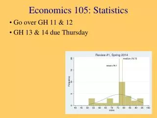
3. Central Limit Theorem Rough statement of CLT: “Sample means are eventually, approximately normally distributed.” Formal statement of CLT: Let X1, X2, X3, . . . ,Xn, where Xiis a random variable denoting the outcome of the ith observation, be an i.i.d. sample from ANY population distribution with mean and variance then as n becomes large Graphically (page 236 in BLK, 10th edition, has a nice visual)

4. CLT!

5. Point and Interval Estimates • A point estimate is a single number, • a confidence interval provides additional information about variability Upper Confidence Limit Lower Confidence Limit Point Estimate Width of confidence interval

6. Point Estimates We can estimate a Population Parameter … with a SampleStatistic (a Point Estimate) μ X Mean π Proportion p

7. Confidence Level, (1-) • Suppose confidence level = 95% • Also written (1 - ) = 0.95 • A relative frequency interpretation: • In repeated samples, 95% of all the confidence intervals that can be constructed are expected to contain the unknown true parameter • A specific interval either will contain or will not contain the true parameter • No probability involved in a specific interval

8. Confidence Intervals Confidence Intervals Population Mean Population Proportion σKnown σUnknown

9. Confidence Intervals for  First, assume 2 is known & X ~ N , so Things are different when these are not true. Random sample of n observations We will use to make inferences about 

10. Confidence Interval for μ(σ Known) • Assumptions • Population standard deviation σis known • Population is normally distributed • Confidence interval estimate:

11. Finding the Critical Value, Z • Consider a 95% confidence interval: Z= -1.96 Z= 1.96 Z units: 0 Lower Confidence Limit Upper Confidence Limit X units: Point Estimate Point Estimate

12. Common Levels of Confidence • Commonly used confidence levels are 90%, 95%, and 99% Confidence Coefficient, Confidence Level Z value 80% 90% 95% 98% 99% 99.8% 99.9% 0.80 0.90 0.95 0.98 0.99 0.998 0.999 1.28 1.645 1.96 2.33 2.58 3.08 3.27

13. The Most Common Confidence Level is 95% +/- 1.96

14. Intervals and Level of Confidence Sampling Distribution of the Sample Mean x Intervals extend from to x1 (1-)x100%of intervals constructed contain μ; ()x100% do not. x2 Confidence Intervals

15. Example • A sample of 11 circuits from a large normal population has a mean resistance of 2.20 ohms. We know from past testing that the population standard deviation is 0.35 ohms. • Determine a 95% confidence interval for the true mean resistance of the population.

16. Example (continued) • A sample of 11 circuits from a large normal population has a mean resistance of 2.20 ohms. We know from past testing that the population standard deviation is 0.35 ohms. • Solution:

17. Interpretations • We are 95% confident that the true mean resistance is between 1.9932 and 2.4068 ohms • True mean may or may not be in this interval • In repeated samples, 95% of confidence intervals formed in this manner are expected to contain the true mean

18. Confidence Intervals Confidence Intervals Population Mean Population Proportion σKnown σUnknown

19. Confidence Interval for μ(σ Unknown) • If the population standard deviation σ is unknown, we can substitute the sample standard deviation, sx • This introduces extra uncertainty, since sx varies from sample to sample • Use t distribution instead of the normal distribution

20. Student’s t distribution William Sealy Gosset was an Irish statistician who worked for Guinness Brewery in Dublin in the early 1900s. He was interested in the effects of various ingredients and temperature on beer, but only had a few batches of each “formula” to analyze. Thus, he needed a way to correctly treat SMALL SAMPLES in statistical analysis. Not supposed to be publishing, so used the pseudonym, “Student”

21. Student’s t distribution • The t is a family of distributions • The shape depends on degrees of freedom (d.f.) • Number of observations that are free to vary after sample mean has been calculated d.f. = n - 1

22. Student’s t distribution Note: t Z as n increases Standard Normal (t with df = ∞) t (df = 13) t-distributions are bell-shaped and symmetric, but have ‘fatter’ tails than the normal t (df = 5) t 0

23. Confidence Interval for μ(σ Unknown) (continued) • Assumptions • Population standard deviation is unknown • Population is normally distributed • Use Student’s t distribution • Confidence Interval Estimate: (where t is the critical value of the t distribution with n -1 degrees of freedom and an area of α/2 in each tail)

24. Student’s t Table Let: n = 3 df = n - 1 = 2  = 0.10/2 = 0.05 Upper Tail Area df .25 .10 .05 1 1.000 3.078 6.314 0.817 1.886 2 2.920 /2 = 0.05 3 0.765 1.638 2.353 The body of the table contains t values, not probabilities 0 t 2.920

25. t distribution values With comparison to the Z value Confidence t t t Z Level (10 d.f.)(20 d.f.)(30 d.f.) ____ 0.80 1.372 1.325 1.310 1.28 0.90 1.812 1.725 1.697 1.645 0.95 2.228 2.086 2.042 1.96 0.99 3.169 2.845 2.750 2.58 Note: t Z as n increases

26. Confidence Intervals for  A manufacturer produces bags of flour whose weights are normally distributed. A random sample of 25 bags was taken and their mean weight was 19.8 ounces with a sample standard deviation of 1.2 ounces. Find and interpret a 99% confidence interval for the true average weight for all bags of flour produced by the company.