GARCH Models and Asymmetric GARCH models
320 likes | 1.64k Vues
GARCH Models and Asymmetric GARCH models. VECM (Review). Cointegrating Eq: R1(-1)1.000000 R10(-1) -0.980444 (0.07657) [-12.8046] C 0.603495 . Error Correction: D(R1) D(R10) CointEq1 -0.029996 0.015287 (0.01783) (0.01140) [-1.68255] [ 1.34155]

GARCH Models and Asymmetric GARCH models
E N D
Presentation Transcript
VECM (Review) • Cointegrating Eq: • R1(-1)1.000000 • R10(-1) -0.980444 • (0.07657) • [-12.8046] • C 0.603495 Error Correction: D(R1) D(R10) CointEq1 -0.029996 0.015287 (0.01783) (0.01140) [-1.68255] [ 1.34155] D(R1(-1)) 0.273219 -0.028276 (0.06803) (0.04348) [ 4.01619] [-0.65026] D(R1(-2)) -0.087596 0.025434 (0.06772) (0.04328) [-1.29358] [ 0.58761] D(R10(-1)) 0.370337 0.425735 (0.10747) (0.06869) [ 3.44593] [ 6.19757] D(R10(-2)) -0.263587 -0.266142 (0.10796) (0.06901) [-2.44152] [-3.85675] C -0.000459
Structure of today’s session • Brief re-cap of last lecture • Estimation of ARCH models • Maximum likelihood estimation • The Glosten Jaganathan and Runkle model which introduces asymmetric adjustment into the model. • Revision
Problems: What value of q should be chosen? The number of lags, q, might be large. The non-negativity constraints might be violated. Generalised ARCH (GARCH) models: Allows the conditional variance, σt2 , to depend its own lags as well as lagged squared residuals. GARCH(1,1) The interpretation here is that the current fitted variance is a weighted function of a long term average value (α0), volatility during the previous period (α1ut-12), and the fitted variance from the model during the previous period (βσt-12).
GARCH Models • The GARCH model is really an ARMA type of process. • To show this the squared residual at time t is equal to the conditional variance and a constant term, to give:
Estimating ARCH/GARCH Models • In practice the likelihood function is expressed in logs (so that a multiplicative function becomes an additive one). • The log-likelihood function (LLF) for an ARCH model with a normally distributed error is given by L: • The computer replaces σ2t in the LLF with its ARCH process.
Maximum Likelihood Estimation: Global maximum L Max Local maximum β βMLE Where L is maximised dlogL/dβ = 0. Software use various algorithms for iteration to the global maximum estimate of β.
ML Estimation of ARCH/GARCH models • Specify the model and its likelihood function • Use OLS regression to get initial estimates (starting values) for β1 , β1 etc. • Choose initial estimates for the parameters of the conditional variance function. Eviews (and other software) offers you zeros as starting values for these. In practice it is better to choose small positive values. • Specify a convergence criteria (usually the software has a default value for this). • Maximise the likelihood by iteration until no further improvement in the model coefficients can be obtained (and the convergence criteria in step 4 is met).
GARCH (p,q): - The current conditional variance depends on q lags of the past squared error and p lags of the past conditional variance. - However higher order models above GARCH(1,1) are rarely used in practice.
Asymmetric GARCH Models • Given that all the terms in a GARCH model are squared, there will always be a symmetric response to positive and negative shocks • However due to the leveraged nature of most firms, a negative shock should be more damaging than a positive shock and therefore produce greater volatility. • There have been two approaches to this stylised fact, the exponential GARCH model and the Glosten, Jagannathan and Runkle models.
Asymmetric Adjustment • The asymmetric adjustment is introduced into the model through the use of a dummy variable which takes the value of 0 or 1 • It takes the value of 1 if the shock is negative (i.e. <0), and 0 otherwise
GJR Model • From the previous slide it is clear that a large positive shock will produce less volatility than a large negative one, assuming the coefficient γ is positive • If the final term is significant, according to the t-statistics, then it implies asymmetric responses are an important effect • The non-negativity constraint for terms 2 and 4 are now:
GJR Model • It is possible to calculate the conditional variance for a positive and negative shock and hence show that these are different. • Clearly in the negative shock case the squared error term will have two components, the individual part and the dummied part.
News Impact Curves • Both GARCH and GJR models can be used to produce plots of the next period volatility, that arises following both positive and negative shocks. • This simply involves substituting values of u(t-1) in the range [-1,+1] into the estimated model, to obtain various values for the conditional variance. • The plot for the GARCH model will be symmetric, for the GJR model, negative shocks will be higher than positive shocks.
EGARCH • The exponential GARCH or EGARCH model was developed by Nelson (1991)taking the following form:
EGARCH • This is the exponential GARCH model and can also be used to explain asymmetries. • A further advantage is that the dependent variable is in logs, so the non-negativity constraint is not breached. • As with the GJR model, if the following term is negative and significant, then there is evidence of asymmetry (the leverage effect):
GARCH-in-mean • This type of model introduces the conditional variance (or standard deviation) into the mean equation. • These are often used in asset return equations, where both return and risk are to be considered. • If the coefficient on this risk variable is positive and significant, it shows that increased risk leads to a higher return. • Similarly it can be introduced into asset parity models, representing the risk premium.
GARCH-in-mean Example • The following model uses the return on a bond as the dependent variable:
GARCH-in-mean Example • In the previous slide, the positive sign and significant t-statistic indicate that the risk of the bond leads to a higher return. • The diagnostic tests are interpreted in the usual way.
Forecasting using GARCH models • The GARCH models are useful for forecasting volatility of asset returns, options and other finance series. • This is particularly important in options pricing, where volatility is an important input into the pricing of the option. • However it is difficult to produce the standard error band for the confidence intervals for the conditional variance forecasts as this requires the variance of the variance.
Forecasting with GARCH • Although the GARCH model has the conditional variance of the error term as its dependent variable, this is the same as the conditional variance of the dependent variable in the mean equation. • This is the case regardless of what variables are included in the mean equation.
Conclusion • The GARCH model is better in general than the ARCH model, as usually a GARCH(1,1) model is sufficient. • The GJR model can be used to model asymmetric adjustment, through the use of a dummy variable. • This allows negative shocks to have higher conditional variance than positive shocks.