Exploring GARCH Models: A Martingale Difference Series Approach with Simulation in R
80 likes | 200 Vues
This document delves into GARCH (Generalized Autoregressive Conditional Heteroskedasticity) models using a martingale difference series. It explores the theoretical aspects and practical implementation through R simulations, demonstrating how to generate a conditional variance structure in a time series. The provided code illustrates the simulation of the series and the resulting plots for data and conditional standard deviation. This analysis contributes to understanding volatility in time series data, particularly in finance, where such models are prevalent.

Exploring GARCH Models: A Martingale Difference Series Approach with Simulation in R
E N D
Presentation Transcript
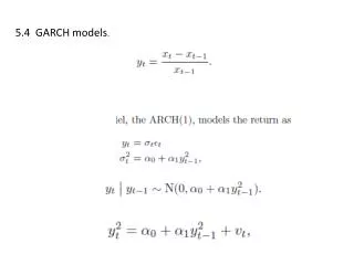
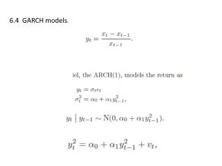
A martingale difference series “Learning a potential function …”
postscript(file="arch.ps",paper="letter",hor=FALSE) par(mfrow=c(2,1)) library(tseries) set.seed(28112006) a0<-1;a1<-.75 ylast<-1;Y<-ylast Sig<-NULL for(i in 1:250){ sig2<-a0+a1*ylast**2 y<-sqrt(sig2)*rnorm(1) ylast<-y Y<-c(Y,y) Sig<-c(Sig,sqrt(sig2)) } plot(Y,type="l",main="Data",xlab="time",ylab="",las=1) plot(Sig,type="l",main="Sig",xlab="time",ylab="",las=1) acf(Y,main="acf of data",xlab="lag",ylab="",las=1) acf(Y**2,main="acf of data-squared",xlab="lag",ylab="",las=1) graphics.off()