Advanced Pathway Simulation in Biological Systems: Insights and Computational Techniques
460 likes | 586 Vues
This lecture covers the complexities of biological pathways and their simulation using molecule-based cell approaches. Prof. Chen Yu Zong explores genomic and proteomic interactions, discussing the dynamics of metabolic networks through graph-theoretic descriptions. He elaborates on degree distribution, scale-free networks, and the mechanisms of growth and preferential attachment that define biological topology. The implications of protein threading and various simulation methodologies are examined, providing insights into the characterizing of complex biological systems.

Advanced Pathway Simulation in Biological Systems: Insights and Computational Techniques
E N D
Presentation Transcript
CZ5225: Modeling and Simulation in BiologyLecture 11: Biological Pathways III: Pathway SimulationProf. Chen Yu ZongTel: 6874-6877Email: yzchen@cz3.nus.edu.sghttp://xin.cz3.nus.edu.sgRoom 07-24, level 7, SOC1, NUS
“Genomes To Life” Computing Roadmap Protein machine Interactions Molecule-based cell simulation Computing and Information Infrastructure Capabilities Molecular machine classical simulation Cell, pathway, and network simulation Community metabolic regulatory, signaling simulations Constrained rigid docking Constraint-Based Flexible Docking Current Computing Genome-scale protein threading Comparative Genomics Biological Complexity
Characterising Pathwaysmetabolic networks as an example To study the network characteristics of the metabolism a graph theoretic description needs to be established. (a) illustrates the graph theoretic description for a simple pathway (catalysed by Mg2+-dependant enzymes). (b) In the most abstract approach all interacting metabolites are considered equally. The links between nodes represent reactions that interconvert one substrate into another. For many biological applications it is useful to ignore co-factors, such as the high-energy-phosphate donor ATP, which results (c) in a second type of mapping that connects only the main source metabolites to the main products. Barabasi & Oltvai, Nature Rev Gen 5, 101 (2004)
Degree The most elementary characteristic of a node is its degree (or connectivity), k, which tells us how many links the node has to other nodes. a In the undirected network, node A has k = 5. b In networks in which each link has a selected direction there is an incoming degree, kin, which denotes the number of links that point to a node, and an outgoing degree, kout, which denotes the number of links that start from it. E.g., node A in b has kin = 4 and kout = 1. An undirected network with N nodes and L links is characterized by an average degree <k> = 2L/N (where <> denotes the average). Barabasi & Oltvai, Nature Reviews Genetics 5, 101 (2004)
Degree distribution The degree distribution, P(k), gives the probability that a selected node has exactly k links. P(k) is obtained by counting the number o f nodes N(k) with k = 1,2... links and dividing by the total number of nodes N. The degree distribution allows us to distinguish between different classes of networks. For example, a peaked degree distribution, as seen in a random network, indicates that the system has a characteristic degree and that there are no highly connected nodes (which are also known as hubs). By contrast, a power-law degree distribution indicates that a few hubs hold together numerous small nodes. Barabasi & Oltvai, Nature Reviews Genetics 5, 101 (2004)
Random networks Aa The Erdös–Rényi (ER) model of a random network starts with N nodes and connects each pair of nodes with probability p, which creates a graph with approximately pN (N-1)/2 randomly placed links. Ab The node degrees follow a Poisson distribution, where most nodes have approximately the same number of links (close to the average degree <k>). The tail (high k region) of the degree distribution P(k ) decreases exponentially, which indicates that nodes that significantly deviate from the average are extremely rare. Ac The clustering coefficient is independent of a node's degree, so C(k) appears as a horizontal line if plotted as a function of k. The mean path length is proportional to the logarithm of the network size, l log N, which indicates that it is characterized by the small-world property. Barabasi & Oltvai, Nature Rev Gen 5, 101 (2004)
Origin of scale-free topology and hubs in biological networks The origin of the scale-free topology in complex networks can be reduced to two basic mechanisms: growth and preferential attachment. Growth means that the network emerges through the subsequent addition of new nodes, such as the new red node that is added to the network that is shown in part a . Preferential attachment means that new nodes prefer to link to more connected nodes. For example, the probability that the red node will connect to node 1 is twice as large as connecting to node 2, as the degree of node 1 (k1=4) is twice the degree of node 2 (k2 =2). Growth and preferential attachment generate hubs through a 'rich-gets-richer' mechanism: the more connected a node is, the more likely it is that new nodes will link to it, which allows the highly connected nodes to acquire new links faster than their less connected peers. Barabasi & Oltvai, Nature Rev Gen 5, 101 (2004)
Scale-free networks Scale-free networks are characterized by a power-law degree distribution; the probability that a node has k links follows P(k) ~ k- -, where is the degree exponent. The probability that a node is highly connected is statistically more significant than in a random graph, the network's properties often being determined by a relatively small number of highly connected nodes („hubs“, see blue nodes in Ba). In the Barabási–Albert model of a scale-free network, at each time point a node with M links is added to the network, it connects to an already existing node I with probability I = kI/JkJ, where kI is the degree of node I and J is the index denoting the sum over network nodes. The network that is generated by this growth process has a power-law degree distribution with = 3. Bb Such distributions are seen as a straight line on a log–log plot. The network that is created by the Barabási–Albert model does not have an inherent modularity, so C(k) is independent of k. (Bc). Scale-free networks with degree exponents 2< <3, a range that is observed in most biological and non-biological networks, are ultra-small, with the average path length following ℓ ~ log log N, which is significantly shorter than log N that characterizes random small-world networks.
Network measures Scale-free networks and the degree exponent Most biological networks are scale-free, which means that their degree distribution approximates a power law, P(k) k-, where is the degree exponent and ~ indicates 'proportional to'. The value of determines many properties of the system. The smaller the value of , the more important the role of the hubs is in the network. Whereas for >3 the hubs are not relevant, for 2> >3 there is a hierarchy of hubs, with the most connected hub being in contact with a small fraction of all nodes, and for = 2 a hub-and-spoke network emerges, with the largest hub being in contact with a large fraction of all nodes. In general, the unusual properties of scale-free networks are valid only for < 3, when the dispersion of the P(k) distribution, which is defined as 2 = <k2> - <k>2, increases with the number of nodes (that is, diverges), resulting in a series of unexpected features, such as a high degree of robustness against accidental node failures. For >3, however, most unusual features are absent, and in many respects the scale-free network behaves like a random one. Barabasi & Oltvai, Nature Reviews Genetics 5, 101 (2004)
Shortest path and mean path length Distance in networks is measured with the path length, which tells us how many links we need to pass through to travel between two nodes. As there are many alternative paths between two nodes, the shortest path — the path with the smallest number of links between the selected nodes — has a special role. In directed networks, the distance ℓAB from node A to node B is often different from the distance ℓBA from B to A. E.g. in b , ℓBA = 1, whereas ℓAB = 3. Often there is no direct path between two nodes. As shown in b, although there is a path from C to A, there is no path from A to C. The mean path length, <ℓ>, represents the average over the shortest paths between all pairs of nodes and offers a measure of a network's overall navigability. Barabasi & Oltvai, Nature Reviews Genetics 5, 101 (2004)
Clustering coefficient In many networks, if node A is connected to B, and B is connected to C, then it is highly probable that A also has a direct link to C. This phenomenon can be quantified using the clustering coefficient CI = 2nI/k(k-1), where nI is the number of links connecting the kI neighbours of node I to each other. In other words, CI gives the number of 'triangles' that go through node I, whereas kI (kI -1)/2 is the total number of triangles that could pass through node I, should all of node I's neighbours be connected to each other. For example, only one pair of node A's five neighbours in a are linked together (B and C), which gives nA = 1 and CA = 2/20. By contrast, none of node F's neighbours link to each other, giving CF = 0. The average clustering coefficient, <C >, characterizes the overall tendency of nodes to form clusters or groups. An important measure of the network's structure is the function C(k), which is defined as the average clustering coefficient of all nodes with k links. For many real networks C(k) k-1, which is an indication of a network's hierarchical character. The average degree <k>, average path length <ℓ> and average clustering coefficient <C> depend on the number of nodes and links (N and L) in the network. By contrast, the P(k) and C(k ) functions are independent of the network's size and they therefore capture a network's generic features, which allows them to be used to classify various networks. Barabasi & Oltvai, Nature Reviews Genetics 5, 101 (2004)
Hierarchical networks To account for the coexistence of modularity, local clustering and scale-free topology in many real systems, it has to be assumed that clusters combine in an iterative manner, generating a hierarchical network. The starting point of this construction is a small cluster of 4 densely linked nodes (4 central nodes in Ca). Next, 3 replicas of this module are generated and the 3 external nodes of the replicated clusters connected to the central node of the old cluster, which produces a large 16-node module. 3 replicas of this 16-node module are then generated and the 16 peripheral nodes connected to the central node of the old module, which produces a new module of 64 nodes. The hierarchical network model seamlessly integrates a scale-free topology with an inherent modular structure by generating a network that has a power-law degree distribution with degree exponent = 1 + ln4/ln3 = 2.26 (Cb) and a large, system-size independent average clustering coefficient <C> ~ 0.6. The most important signature of hierarchical modularity is the scaling of the clustering coefficient, which follows C(k) ~ k-1 a straight line of slope -1 on a log–log plot (Cc). A hierarchical architecture implies that sparsely connected nodes are part of highly clustered areas, with communication between the different highly clustered neighbourhoods being maintained by a few hubs (Ca). Barabasi & Oltvai, Nature Rev Gen 5, 101 (2004)
Constructing a pathway model:things to consider 1.Dynamic nature of biological networks. Biological pathway is more than a topological linkageof molecular networks. Pathway models can be based on network characteristics including those of invariant features.
Constructing a pathway model:things to consider 2.Abstraction Resolution: • How much do we get into details? • What building blocks do we use to describe the network? High resolution Low resolution (A) Substrates and proteins (B) Pathways (C) “special pathways”
Constructing a pathway modelStep I - Definitions We begin with a very simple imaginary metabolic network represented as a directed graph: How do we define a biologically significant system boundary? Vertex – protein/substrate concentration. Edge - flux (conversion mediated by proteins of one substrate into the other) Internal flux edge External flux edge
Constructing a pathway modelStep II - Dynamic mass balance Concentration vector Stoichiometry Matrix Flux vector
A model pathway system and its time-dependent behavior Positive Feedback Loop
A model pathway system and its time-dependent behavior
A model pathway system and its time-dependent behavior
Constructing a pathway modelStep II - Dynamic mass balance • Problem … Concentration vector Stoichiometry Matrix Flux vector V=V(k1, k2,k3…) is actually a function of concentration as well as several kinetic parameters. it is very difficult to determine kinetic parameters experimentally. Consequently there is not enough kinetic information in the literature to construct the model. • One Solution: In order to identify invariantcharacteristics of the network, one can assume the network is at steady state.
Constructing a pathway modelStep III - Dynamic mass balance at steady state • What does “steady state” mean? • 2. Is it biologically justifiable to assume it? • 3. Does it limit the predictive power of pathway model? “The steady state approximation is generally valid for some metabolic pathways because of fast equilibration of metabolite concentrations (seconds) with respect to the time scale of genetic regulation (minutes)” – Segre 2002 How about signaling pathways?
How can the steady state assumption solve pathway simulation problem? Steady state assumption
£ b 0 j Constraints on external fluxes: Source Sink Sink/source is unconstrained In other words flux going into the system is considered negative while flux leaving the system is considered positive. Remark: further constraints can be imposed both on the internal flux as well as the external flux… Constructing a pathway modelStep IV - Adding constraints Constraints on internal fluxes:
Flux cone and metabolic capabilities Observation: the number of reactions considerably exceeds the number of metabolites The S matrix will have more columns than rows The null space of viable solutions to our linear set of equations contains an infinite number of solutions. What about the constraints? “The solution space for any system of linear homogeneous equations and inequalities is a convexpolyhedral cone.” - Schilling 2000 C Our flux cone contains all the points of the null space with non negative coordinates (besides exchange fluxes that are constrained to be negative or unconstrained)
Flux cone and metabolic capabilities • What is the significance of the flux cone? • It defines what the network can do and cannot do! • Each point in this cone represents a flux distribution in which the system can operate at steady state. • The answers to the following questions (and many more) are found within this cone: • what are the building blocks that the network can manufacture? • how efficient is energy conversion? • Where is the critical links in the system?
Navigating through the flux cone byusing “Extreme pathways” • Next thing to do is develop a way to describe and interpret any location within this space. • We will not use the traditional reaction/enzyme based perspective • Instead we use a pathway perspective: Extreme rays - “extreme rays correspond to edges of the cone. They are said to generate the cone and cannot be decomposed into non-trivial combinations of any other vector in the cone.”- schilling 2000 What is the analogy in linear algebra? We use the termExtreme Pathwayswhen referring to Extreme rays of a convex polyhedral cone that represents metabolic fluxes • Differences • Unlike a basis the set of, extreme pathways is typically unique • Any flux in the cone can be described using a non negative combination of extreme rays.
C v Navigating through the flux cone byusing “Extreme pathways” • Extreme Pathways will be denoted by vector EPi (0≤ i ≤ k) • Every point within the cone can be written as a non-negative linear combination of the extreme pathways. In biological context this means that : any steady state flux distribution can be represented by a non-negative linear combination of extreme pathways.
Compute steady state flux Convex + constraints Identify Extreme pathways (using algorithm presented in Schilling 2000) The entire process from a bird’s eye view
Lets look at a specific vector v’ : Is v inside the flux cone? Easy to check… 1. Does v fulfill constraints? 2. Is v in the null space of Sv=0 ? Example
P v w = = • v’=4*p1+1*p2+1*p3 Example can v be represented by using a non-negative linear combination of extreme pathways ? We can reformulate this concept using matrix notation: The vector w gives us a pathway based perspective of the network functioning!
Flux Balance Analysis • Simulates Flux or Flow through Metabolic Pathways • Kinetics of each step not required • Predicts effects of gene knockouts
The Multiscale Problem in Systems Biology In the heat-shock response in E. Coli, an estimated 20 - 30 sigma-32 molecules per cell play a key role in sensing the folding state of the cell and in regulating the production of heat shock proteins. The system cannot be simulated at the fully stochastic level due to: • Multiple time scales (stiffness) • The presence of exceedingly large numbers of molecules that must be accounted for in SSA
Computational Models of Molecular Networks • Discrete and stochastic - Finest scale of representation for well stirred molecules. Exact description via Stochastic Simulation Algorithm (SSA) due to Gillespie. This is the method described here • Continuous and stochastic - The Langevin regime. Valid under certain conditions. Described by Stochastic Differential Equations (SDE). • Continuous and deterministic - The chemical rate equations. Described by ordinary differential equations (ODE). Valid under further assumptions.
Stochastic Simulation Algorithm • Well-stirred mixture • N molecular species • Constant temperature, fixed volume • M reaction channels • Dynamical state where is the number of molecules in the system
Stochastic Simulation Algorithm • Propensity function the probability, given , that one reaction will occur somewhere inside in the next infinitesimal time interval • When that reaction occurs, it changes the state. The amount by which changes is given by the change in the number of molecules produced by one reaction • is a jump Markov process
Stochastic Simulation Algorithm • Draw two independent samples and from and take the smallest integer satisfying • Update X
Hybrid Methods • Slow reactions involving species present in small numbers are simulated by SSA • Reactions where all constituents present with large populations are simulated by reaction-rate equations Haseltine and Rawlings, 2002 Matteyses and Simmons, 2002 What to do about other scenarios???
A Closer Look at the Multiscale Challenges for Heat Shock Response The total “concentration” of 32 is 30-100 per cell But the “concentration” of free 32 is .01-.05 per cell DNAK RNAP RNAP DnaK FtsH
Stochastic Partial Equilibrium Approximation • In deterministic simulation of chemical systems, the partial equilibrium approximation assumes that the fast reactions are always in equilibrium. These fast reactions are thus treated as algebraic constraints. • In stochastic simulation, the states keep changing. The stochastic partial equilibrium approximation is based on the assumption that the distributions of the fast species remain unchanged by the fast reactions. • Partition and re-index reactions so that are fast reactions and are slow reactions. Partition the species so that are fast species (any species involved in at least one fast reaction), and are slow species • The virtual system with only fast reactions and fast species is assumed to be in stochastic partial equilibrium, on the time scale of the slow reactions
Foundations of SPEA • Let the probability that, given , no slow reaction fires during . • Define . • We will not simulate the fast reactions. Instead we take attime as a random variable. The probability that one slowreaction will occur in is given by where mean over only.
Foundations of SPEA • Let be so small that in the next at most one slow reaction could fire. • Then (1) • Solving (1) we obtain (2) • Define the next slow reaction density function as the probability that, given , the next slow reaction will occur in and will be an reaction. Then (2) leads to (3) • Now apply the stochastic partial equilibrium approximation. Assume the virtual system is at partial equilibrium and is small compared to . Then can be taken as . • Thus
The Multi-scale Stochastic Simulation Algorithm Given initial time , initial state and final simulation time , • Compute the partial equilibrium state for the fast reaction channels. This involves solving a nonlinear system arising from the equilibrium approximation and the local conservation laws for 2. For , calculate and . (This is the most difficult task) 3. Generate two random numbers and from . The time for the next slow reaction to fire is given by , where . The index of the next slow reaction is the smallest integer satisfying . 4. If , stop. Otherwise, update .
Down-Shifting Method • The MSSA method captures the full distribution information for the slow species, but computes only the mean accurately for the fast species. • However, the distribution information of the fast species can be easily recovered by taking a few small time steps whenever this information is needed. • This ‘down-shifting’ works because the system is a Markov process!
Heat Shock Response Model • Stochastic Model involves 28 species and 61 chemical reactions. This is a moderate-sized model. • CPU time on 1.46 Ghz Pentium IV Linux workstation for one SSA simulation is 90 seconds. • CPU time for 10,000 simulations is more than 10 days. • 12 fast reactions were chosen for the SPEA. The fast reactions were identified from a single SSA simulation to be the ones that fired most frequently. These 12 reactions fire 99% of the total number of times for all reaction channels. • CPU time for the multiscale SSA • Without down-shifting: 3 hours for 10,000 runs • With down-shifting: 4 hours for 10,000 runs
MSSA Heat Shock Response Model Results Histogram (10,000 samples) of a slow species mRNA(DNAK) (left) and a fast species DNAK with (right) and without downshifting method (middle) solved by the original SSA method (purple solid line with ‘o’) and the MSSA method (red dashed line with ‘+’), for the HSR model. fast species with down shifting one slow species one fast species