Random Graph Model for Internet Worm Epidemics
Presentation on using random graphs to model the spread of computer worms in the Internet, discussing scale-free networks, epidemic models, and their relationship. Explore Aiello et al.'s random graph model for SF graphs. Graph theory in epidemic studies.

Random Graph Model for Internet Worm Epidemics
E N D
Presentation Transcript
A Model Using Random Graph Theory PRESENTED TO: CSIIR WorkshopOak Ridge National Lab PRESENTED BY*: Christopher Griffin Penn State Applied Research *Richard R. Brooks of Clemson University contributed to this study.
Goals of Presentation • Summarize the epidemiological models of worm spread in the Internet • Introduce Random Graphs as models of the Internet • Propose a natural model of worm spread using Random Graphs • Demonstrate quantitative results showing this model may be appropriate
Computer Worms • Computing a self-replicating program able to propagate itself across a network, typically having a detrimental effect. • The name 'worm' comes from The Shockwave Rider, a science fiction novel published in 1975 by John Brunner. • Researchers John F Shoch and John A Hupp of Xerox PARC chose the name in a paper published in 1982; The Worm Programs, Comm ACM, 25(3):172-180, 1982), and it has since been widely adopted.
Epidemic Models • Epidemiology: The study of the spread of disease in populations. • Diseases may spread quickly and then die out (Ebola) or remain endemic within a population (Chicken Pox) • Populations can be modeled in a number of ways: • “SI”, “SIS” or “SIR” models are most common.
Mathematical Epidemiology • Classical Mathematical Epidemiology Uses 3 Key Parameters in SIS/SIR Models: • R0: The number of secondary infections that occur when one infective agent is introduced into a population. • (t): The average number of effective contacts an individual has during his/her infected period. • R(t) : The average number of secondary infections produced by an individual during his/her infected period. • In general, epidemic is only possible if R0 > 1.
Scale-Free Networks • A graph G=(V,E) is scale free if the number of vertices with degree d follows an inverse power law. That is: • n(d) = k/d • n(d) is the number of vertices with degree d. • k is a constant of proportionality, and • is the scaling parameter. • Scale-free graphs have gained popularity in recent years. • Examples: The World Wide Web, Human Sexual Contacts, Protein-Protein Interaction Networks.
Worm Models with Epidemiology • R. Pastor-Satorras and A. Vespigani studied the spread of worms in Internet-like networks using classical mathematical epidemiology. • Differential Equation Model of Infection Spread • Mean-Field Theory Approximations • They show that for certain scale-free networks with scaling parameter < 3, epidemics will occur for all diseases with R0 > 1.
OK, this model “looks” good. Why not use it? • Three reasons to search for a different model: • These models assume a completely mixed population. • Classical mathematical epidemiology assumes a fluid-like behavior of individuals. • R. Pastor-Satorras and A. Vespigani were studying general scale-free networks, not computer networks specifically. • Two dangers to note: • In the absence of ad hoc mesh networks, computers do not mix. • The effective R0 is highly dependent on the initial infection position.
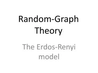
Graphs and Random Graphs • A graph G=(V,E) is said to have a giant component H if H is a subgraph and contains a majority of the vertices of G. • A random graph is a misnomer. A random graph is a tuple (,p), where is a set of graphs and p is an appropriately defined probability measure on a sigma algebra of . • The most widely studied random graph family is (n,p), where each graph in has n vertices when any graph G is chosen from the probability that there is an edge between two arbitrarily chosen vertices is p. • These are the Erdös-Renyi Random Graphs.
Random Graph Model of SF Graphs • Aiello et al. have formulated a random graph model of SF graphs. • Let (,) be the collection of graphs whose degree distribution follows the curve n(d)=exp()/d. • Here xdenotes the greatest integer lower bound for x. • Aiello et al. have shown that this definition is mathematically sufficient and that a reasonable probability measure can be defined. • In this model, (roughly) controls the size of the graph while controls the scaling of the graph.
Relation to Epidemic Models • Lemma [Griffin & Brooks 2006]: If G is an element of (,), and vertices of G are uniformly randomly kept with probability 0<p≤1 to produce G’, then a.s. G’ has the same properties as G. • Theorem [Griffin & Brooks 2006]: For any infection in graph G(,) with >2, and with nodes having susceptibility probability p, then for all time
Infection Potential • Theorem [Griffin & Brooks 2006]: If 2<<0, and for any infectious agent with infection probability p, a.s. limti(t) = p. Where i(t) is the proportion of infected nodes. • This result is particularly interesting: • Often the affects of Internet worms have been blamed on the monoculture of Microsoft products. • This theorem suggests that even in the absence of a network monoculture, for appropriate Internet structures, 100% infection would occur among the susceptible nodes.
Rate of Infection • Theorem [Griffin & Brooks]: Suppose that the rate of infection is constant, then the time required to achieve total infection is a.s. O(log|G|). • Suppose that the infection rate is r(t), then: • For certain r(t) we can obtain an “S” curve matching the data. • This gives a natural model of infection rate that matches the given data and does not appeal to continuous mixing models.
Comparison of Approaches • When we try a model: • We obtain: • The model is seen to be imperfect because the true “logarithmic rate” does have hump, but it is probably not Gaussian in nature. • G/B puts the diameter of this monitored network at ~13--this is a bit smaller than most estimates of the diameter of the Internet.
Infection Countermeasures • Theorem [Griffin & Brooks 2006]: Centralized patch distribution runs in O(|G|), while decentralized “white worms” can inoculate machines in time O(log|G|) assuming a constant rate of transmission. • This theorem was “experimentally verified” by Chen and Carley (2005). • What does this mean? • Centralized patch distribution is inefficient but… • Centralized patch distribution is safe. • Inefficiency is the cost of safety. • Here is a real tradeoff: either we distribute patches quickly and prevent global infection at the risk of creating patch-based errors or we live with our current security model.
Conclusions • Infectious agents in computer networks can be modeled using natural “random graph” models. • These models are more appropriate than continuous mixing models. • For scale-free random graph models, total infection is a.s. whenever <0, hence infections are a function of network structure as much as pathogen. • Infection rates can be well described using the random graph model. • There is a natural trade-off between security countermeasures efficiency and safety. This confirms experimental results presented by Chen and Carley.