Understanding Benefit-Cost Analysis in Civil Systems Planning Courses
200 likes | 334 Vues
This lecture explores benefit-cost analysis in civil systems planning through real-world car comparisons and decision-making models. Key concepts include trade-offs based on fuel efficiency, comfort, and pricing, emphasizing the importance of understanding one's willingness to trade different attributes. Additionally, the lecture delves into first-order and second-order stochastic dominance, comparing payoffs of options, and their implications in risk management and decision-making. Students will be equipped with essential tools to evaluate complex projects effectively.

Understanding Benefit-Cost Analysis in Civil Systems Planning Courses
E N D
Presentation Transcript
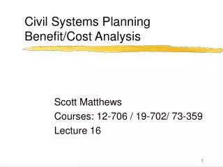
Civil Systems PlanningBenefit/Cost Analysis Scott Matthews Courses: 12-706 / 19-702/ 73-359 Lecture 16
Admin • Project 1 - avg 85 (high 100) • Mid sem grades today - how done? 12-706 and 73-359
Recall: Choosing a Car Example • Car Fuel Eff (mpg) Comfort • Index • Mercedes 25 10 • Chevrolet 28 3 • Toyota 35 6 • Volvo 30 9 12-706 and 73-359
“Pricing out” • Book uses $ / unit tradeoff • Our example has no $ - but same idea • “Pricing out” simply means knowing your willingness to make tradeoffs • Assume you’ve thought hard about the car tradeoff and would trade 2 units of C for a unit of F (maybe because you’re a student and need to save money) 12-706 and 73-359
With these weights.. • U(M) = 0.26*1 + 0.74*0 = 0.26 • U(V) = 0.26*(6/7) + 0.74*0.5 = 0.593 • U(T) = 0.26*(3/7) + 0.74*1 = 0.851 • U(H) = 0.26*(4/7) + 0.74*0.6 = 0.593 • Note H isnt really an option - just “checking” that we get same U as for Volvo (as expected) 12-706 and 73-359
MCDM - Swing Weights • Use hypothetical combinations to determine weights • Base option = worst on all attributes • Other options - “swings” one of the attributes from worst to best • Determine your rank preference, find weights 12-706 and 73-359
Add 1 attribute to car (cost) • M = $50,000 V = $40,000 T = $20,000 C=$15,000 • Swing weight table: • Benchmark 25mpg, $50k, 3 Comf 12-706 and 73-359
Stochastic Dominance “Defined” • A is better than B if: • Pr(Profit > $z |A) ≥ Pr(Profit > $z |B), for all possible values of $z. • Or (complementarity..) • Pr(Profit ≤ $z |A) ≤ Pr(Profit ≤ $z |B), for all possible values of $z. • A FOSD B iff FA(z) ≤ FB(z) for all z 12-706 and 73-359
Stochastic Dominance:Example #1 • CRP below for 2 strategies shows “Accept $2 Billion” is dominated by the other. 12-706 and 73-359
Stochastic Dominance (again) • Chapter 4 (Risk Profiles) introduced deterministic and stochastic dominance • We looked at discrete, but similar for continuous • How do we compare payoff distributions? • Two concepts: • A is better than B because A provides unambiguously higher returns than B • A is better than B because A is unambiguously less risky than B • If an option Stochastically dominates another, it must have a higher expected value 12-706 and 73-359
First-Order Stochastic Dominance (FOSD) • Case 1: A is better than B because A provides unambiguously higher returns than B • Every expected utility maximizer prefers A to B • (prefers more to less) • For every x, the probability of getting at least x is higher under A than under B. • Say A “first order stochastic dominates B” if: • Notation: FA(x) is cdf of A, FB(x) is cdf of B. • FB(x) ≥ FA(x) for all x, with one strict inequality • or .. for any non-decr. U(x), ∫U(x)dFA(x) ≥ ∫U(x)dFB(x) • Expected value of A is higher than B 12-706 and 73-359
FOSD 12-706 and 73-359 Source: http://www.nes.ru/~agoriaev/IT05notes.pdf
Option A Option B FOSD Example 12-706 and 73-359
Second-Order Stochastic Dominance (SOSD) • How to compare 2 lotteries based on risk • Given lotteries/distributions w/ same mean • So we’re looking for a rule by which we can say “B is riskier than A because every risk averse person prefers A to B” • A ‘SOSD’ B if • For every non-decreasing (concave) U(x).. 12-706 and 73-359
Option A Option B SOSD Example 12-706 and 73-359
Area 2 Area 1 12-706 and 73-359
SOSD 12-706 and 73-359
SD and MCDM • As long as criteria are independent (e.g., fun and salary) then • Then if one alternative SD another on each individual attribute, then it will SD the other when weights/attribute scores combined • (e.g., marginal and joint prob distributions) 12-706 and 73-359
Reading pdf/cdf graphs • What information can we see from just looking at a randomly selected pdf or cdf? 12-706 and 73-359