Download
1 / 31
310 likes | 531 Vues
Part09: Applications of Multi-level Models to Spatial Epidemiology. Francesca Dominici & Scott L Zeger. Outline. Multi-level models for spatially correlated data Socio-economic and dietary factors of pellagra deaths in southern US Multi-level models for geographic correlation studies

E N D
Part09: Applications of Multi-level Models to Spatial Epidemiology Francesca Dominici & Scott L Zeger
Outline • Multi-level models for spatially correlated data • Socio-economic and dietary factors of pellagra deaths in southern US • Multi-level models for geographic correlation studies • The Scottish Lip Cancer Data • Multi-level models for air pollution mortality risks estimates • The National Mortality Morbidity Air Pollution Study
Data characteristics • Data for disease mapping consists of disease counts and exposure levels in small adjacent geographical area • The analysis of disease rates or counts for small areas often involves a trade-off between statistical stability of the estimates and geographic precision
An example of multi-level data in spatial epidemiology • We consider approximately 800 counties clustered within 9 states in southern US • For each county, data consists of observed and expected number of pellagra deaths • For each county, we also have several county-specific socio-economic characteristics and dietary factors • % acres in cotton • % farms under 20 acres • dairy cows per capita • Access to mental hospital • % afro-american • % single women
Definition of Pellagra • Disease caused by a deficient diet or failure of the body to absorb B complex vitamins or an amino acid. • Common in certain parts of the world (in people consuming large quantities of corn), the disease is characterized by scaly skin sores, diarrhea, mucosal changes, and mental symptoms (especially a schizophrenia-likedementia). It may develop after gastrointestinal diseases or alcoholism.
Crude Standardized Mortality Ratio (Observed/Expected) of Pellagra Deaths in Southern USA in 1930 (Courtesy of Dr Harry Marks)
Scientific Questions • Which social, economical, behavioral, or dietary factors best explain spatial distribution of pellagra in southern US? • Which of the above factors is more important for explaining the history of pellagra incidence in the US? • To which extent, state-laws have affected pellagra?
Statistical Challenges • For small areas SMR are very instable and maps of SMR can be misleading • Spatial smoothing • SMR are spatially correlated • Spatially correlated random effects • Covariates available at different level of spatial aggregation (county, State) • Multi-level regression structure
Spatial Smoothing • Spatial smoothing can reduce the random noise in maps of observable data (or disease rates) • Trade-off between geographic resolution and the variability of the mapped estimates • Spatial smoothing as method for reducing random noise and highlight meaningful geographic patterns in the underlying risk
Shrinkage Estimation • Shrinkage methods can be used to take into account instable SMR for the small areas • Idea is that: • smoothed estimate for each area “borrow strength” (precision) from data in other areas, by an amount depending on the precision of the raw estimate of each area
Shrinkage Estimation • Estimated rate in area A is adjusted by combining knowledge about: • Observed rate in that area; • Average rate in surrounding areas • The two rates are combined by taking a form of weighted average, with weights depending on the population size in area A
Shrinkage Estimation • When population in area A is large • Statistical error associated with observed rate is small • High credibility (weight) is given to observed estimate • Smoothed rate is close to observed rate • When population in area A is small • Statistical error associated with observed rate is large • Little credibility (low weight) is given to observed estimate • Smoothed rate is “shrunk” towards rate mean in surrounding areas
SMR of pellagra deaths for 800 southern US counties in 1930 Smoothed SMR Crude SMR
Multi-level Models for Geographical Correlation Studies • Geographical correlation studies seek to describe the relationship between the geographical variation in disease and the variation in exposure
Example: Scottish Lip Cancer Data(Clayton and Kaldor 1987 Biometrics) • Observed and expected cases of lip cancer in 56 local government district in Scotland over the period 1975-1980 • Percentage of the population employed in agriculture, fishing, and forestry as a measure of exposure to sunlight, a potential risk factor for lip cancer
Crude standardized Mortality rates for each district, Note that there is a tendency for areas to cluster, with a noticeable grouping of areas with SMR> 200 to the North of the country
Model B: Local Smoothing Crude SMR Smoothed SMR
Posterior distribution of Relative Risksfor maximum exposure B: Local smoothing (posterior mean = 2.18) A: Global smoothing (posterior mean = 3.25)
Posterior distribution of Relative Risksfor average exposure B: Local smoothing (posterior mean=1.09) A: Global smoothing (posterior mean = 1.08)
Results • Under a model for global smoothing, the posterior mean of the relative risk for lip cancer in areas with the highest percentage of outdoor workers is 3.25 • Under model for local smoothing, the posterior mean is lower and equal to 2.18
Discussion • In multi-level models is important to explore the sensitivity of the results to the assumptions inherent with the distribution of the random effects • Specially for spatially correlated data the assumption of global smoothing, where the area-specific random effects are shrunk toward and overall mean might not be appropriate • In the lip cancer study, the sensitivity of the results to global and local smoothing, suggest presence of spatially correlated latent factors
Discussion • Multilevel models are a natural approach to analyze data collected at different level of spatial aggregation • Provide an easy framework to model sources of variability (within county, across counties, within regions etc..) • Allow to incorporate covariates at the different levels to explain heterogeneity within clusters • Allow flexibility in specifying the distribution of the random effects, which for example, can take into account spatially correlated latent variables
Key Words • Spatial Smoothing • Disease Mapping • Geographical Correlation Study • Hierarchical Poisson Regression Model • Spatially correlated random effects • Posterior distributions of relative risks