Bayesian Networks for Modeling Gene Expression Data
Bayesian Networks for Modeling Gene Expression Data. Sushmita Roy BMI/CS 576 www.biostat.wisc.edu/bmi576 sroy@biostat.wisc.edu Nov 19 th , 2013. Bayesian networks (BN). A BN compactly represents a joint probability distribution It has two parts: A graph which is directed and acyclic

Bayesian Networks for Modeling Gene Expression Data
E N D
Presentation Transcript
Bayesian Networks for Modeling Gene Expression Data Sushmita Roy BMI/CS 576 www.biostat.wisc.edu/bmi576 sroy@biostat.wisc.edu Nov 19th, 2013
Bayesian networks (BN) • A BN compactly represents a joint probability distribution • It has two parts: • A graph which is directed and acyclic • A set of conditional distributions • Directed Acyclic Graph (DAG) • The nodes denote random variables X1… XN • The edges • encode statistical dependencies between the random variables • Establish parent child relationships • Each node Xi has a conditional probability distribution (CPD) representing P(Xi| Parents(Xi)) • Provides a tractable way to work with large joint distributions • The joint is written as a product of “local” conditional distributions, one per Xi
Bayesian network representation of a regulatory network Random variables encode expression levels Regulators (Parents) X2 X1 X1 Sho1 X2 Msb2 P(X3|X1,X2) X3 Target (child) X3 Ste20 Parameters of CPD for child given parents. Structure Genes Random variables
Bayesian networks compactly represent joint distributions CPD
Example Bayesian network of 5 variables Parents X2 X1 X4 X3 Child X5 Assume Xi is binary Needs 25 measurements No independence assertions Needs 23 measurements Independence assertions
CPD in Bayesian networks • The same structure can be parameterized in different ways • For example for discrete variables we can have table or tree representations
Representing CPDs as tables • Consider the following case with Boolean variablesX1, X2, X3, X4 P( X4|X1, X2,X3 ) as a table X4 Parents of X4 X2 X1 X3 X4
Estimating CPD table from data • Consider the four RVs from the previous slide • Assume we observe the following data X1 X2 X3 X4 For each joint assignment to X1, X2, X3, estimate the probabilities for each possible value of X4 For example, consider X1=T, X2=F, X3=T P(X4=T|X1=T, X2=F, X3=T)=2/4 P(X4=F|X1=T, X2=F, X3=T)=2/4
P( X4|X1, X2,X3 ) as a tree X1 f t Pr(X4=t) = 0.9 X2 f t Pr(X4=t) = 0.5 X3 f t Pr(X4=t) = 0.8 Pr(X4=t) = 0.5 A tree representation of a CPD Parents of X4 X2 X1 X3 X4 Allows more compact representation of CPDs. For example, we can ignore some quantities.
The learning problems • Parameter learning on known structure • Given training data D, estimate parameters of the conditional distributions • Structure learning • Given training data D, find the statistical dependency structure, G and parameters that best describe D • Subsumes parameter learning
Structure learning using score-based search ... Data Bayesian network Maximum likelihood parameters
Learning network structure is computationally expensive • For N variables there are possible networks: • Set of possible networks grows super exponentially Need approximate methods to search the space of networks
Heuristic search of Bayesian network structures • Make local changes to the network • Add an edge • Delete an edge • Reverse an edge • Evaluate score and select the network configuration with best score • We just need to check for cycles • Working with gene expression data requires additional considerations
D D D C C C B B B A A A Structure search operators Current network add an edge delete an edge Check for cycles
Decomposability of scores • Score of a graph G decomposes over individual variables • This enables us to efficiently compute the score effect of local changes • However, network inference from expression data is very challenging • Lots of nodes and not enough data • Good heuristics to prune the search space are highly desirable • Assess statistical significance of learned network structures
Extensions to Bayesian networks to handle large number of random variables • Sparse candidate algorithm • Bootstrap-based ideas to score high confidence network • Module networks (subsequent lecture)
The Sparse candidate Structure learning in Bayesian networks • Key idea: Identify k promising “candidate” parents for each network based on local measures such as correlation/mutual information • k<<N, N: number of random variables. • Restrict networks to only include a subset of the “candidate” set. • Possible pitfall • Early choices might exclude other good parents • Resolve using an iterative algorithm Friedman, 1999
Sparse candidate algorithm notation • Bn: Bayesian network at iteration n • Cin: Candidate parent set for node Xi at iteration n • Pan(Xi): Parents ofXiinBn
Sparse candidate algorithm • Input: • A data set D • An initial network B0 • A parameter k: number of parents • Output: • Network B • Loop until convergence • Restrict • Based on D and Bn-1 select candidate parents Cin-1 for variable Xi • This defines a skeleton directed network Hn • Maximize • Find network Bn that maximizes the score Score(Bn;D) among networks satisfying • Termination: Return Bn
The Restrict Step Measures of relevance
Information theoretic concepts • KullbackLeibler (KL) Divergence • Distance between two distributions • Mutual information • Mutual information between two random variables X and Y measures statistical dependence between X and Y • Also the KL Divergence between the P(X,Y) and P(X)P(Y) • Conditional Mutual information • Measures the information between two variables given a third
KL Divergence P(X), Q(X) are two distributions over X
Mutual Information • Measure of statistical dependence between two random variables, X and Y • KL Divergence between the joint and product of marginals • DKL(P(X,Y)||P(X)P(Y))
Conditional Mutual Information Measures the mutual information between X and Y, given Z If Z captures everything about X, knowing Y gives no more information about X. Thus the conditional mutual information would be zero.
Measuring relevance of candidate parents in the Restrict Step • A good parent for node Xi is one that has a strong statistical dependence with Xi • Mutual information provides a good measure of statistical dependence I(Xi; Xj) • Mutual information should be used only as a first approximation • Candidate parents need to be iteratively refined to avoid missing important dependences
D C B A Mutual information can miss some parents • Consider the following true network • If I(A;C)>I(A;D)>I(A;B) and we are selecting two candidate parents, B will never be selected as a parent • How do we get B as a candidate parent? • Note if we used mutual information alone to select candidates, we might be stuckwith C and D
Sparse candidate restrict step • Three strategies to handle the effect of greedy choices in the beginning • One can estimate the discrepancy between the (in)dependencies in the network vs those in the data • KL Divergence between P(A,D) in the data vs P(A,D) from the network. • Measure how much the current parent set shields A from D • Conditional mutual information between A and D given the current parent set of A. • Measure how much the score improves on adding D
Measuring relevance of Y to X • MDisc(X,Y) • DKL(P(X,Y)||PB(X,Y)) • MShield(X,Y) • I(X;Y|Pa(X)) • Mscore(X,Y) • Score(X;Y,Pa(X),D)
Performance of Sparse candidate over simple hill-climbing Score 15 seems to perform the best Dataset 2 Dataset 1 200 variables 100 variables
Assessing confidence in the learned network • Given the large number of variables and small datasets, the data is not sufficient to reliably determine the “best” network • One can however estimate the confidence of specific properties of the network • Graph features f(G) • Examples of f(G) • An edge between two random variables • Order relations: Is X Y’s ancestor? • Is X in the Markov blanket of Y • Markov blanket of Y is defined as those variables that render Y independent from the rest of the network • Includes Y’s parents, children and parents of Y’s children
B C D A F E Markov blanket • If MB(X) is the Markov blanket of X then P(X|MB(X),Y)=P(X|MB(X)). X X’s Markov blanket
How to assess confidence in graph features? • What we want is P(f(G)|D), which is • But it is not feasible to compute this sum • Instead we will use a “bootstrap” procedure
Bootstrap to assess graph feature confidence • Fori=1 to m • Construct dataset Di by sampling with replacement N samples from dataset D, where N is the size of the original D • Learn a network Gi • For each feature of interest f, calculate confidence
randomize each row independently Does the confidence estimated from bootstrap procedure represent real relationships? • Compare the confidence distribution to that obtained from randomized data • Shuffle the columns of each row (gene) separately. • Repeat the bootstrap procedure conditions genes
Application of Bayesian network to yeast expression data • 76 experiments/microarrays • 800 genes • Bootstrap procedure on 200 subsampled datasets • Sparse candidate as the Bayesian network learning algorithm
Bootstrap-based confidence differs between original and randomized data --- Randomized data Original data
Example of a high confidence sub-network One learned Bayesian network Bootstrapped confidence Bayesian network Highlights a subnetwork associated with yeast mating
Summary • Network inference from expression provides a promising approach to identify cellular networks • Bayesian networks are one representation of networks that have a probabilistic and graphical component • Network inference naturally translates to learning problems in Bayesian networks. • Network inference is computationally challenge • Successful application of Bayesian network learning algorithms to expression data requires additional considerations • Reduce potential parents: statistically or using biological knowledge • Bootstrap based confidence estimation • Permutation based assessment of confidence