Modeling of Gene expression

1. Modeling of Gene expression . Central Dogma of Molecular Biology : Cell processes Transcription factors Proteins mRNA Gene

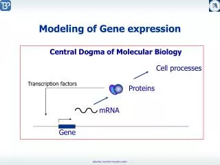
2. Modeling of Gene Expression • Modeling of Expression of one/few genes • Binding of transcription factors/RNAPolymerasen,... to DNA • Effect of inhibitors/activators • Production of mRNA, proteins • Feedback or regulation by products or external regulators Basis: Processes and interactions • Discovery of genetic networks • - Cause of gene expression patterns or -profils • Modeling of the dynamics of artifical networks • Reverse Engineering • Search for Motifs and Clustern Basis: Data

3. Direction of Investigation known to be predicted Structure Function Protein interactions Expression of genes TF bindiung Regulation Impact of perturbations Dynamic behavior, Bifurcations,... : : Function Structure Expression patternMutual influence of genes Time courses of Regulation network concentrations, activities,…. : :

4. Concept of state The state of a system is a snapshot of the system at a given time that contains enough information to predict the behaviour of the system for all future times. The state of the system is described by the set of variables that must kept track of in a model. Different models of gene regulation have different representations of the state: Boolean model: a state is a list containing for each gene involved, of whether it is expressed („1“) or not expressed („0“) Differential equation model: a list of concentrations of each chemical entity Probabilistic model: a current probability distribution and/or a list of actual numbers of molecules of a type Each model defines what it means by the state of a system. Given the current state the model predicts what state/s can occur next.

5. Deterministic, continuous time and state: e.g. ODE model concentration of A decreases and concentration of B increases. Concentration change in per time interval dtis given by Probabilistic, discrete time and state : transformation of a molecule of type A into a molecule of type Sorte B. The probability of this event in a time interval dtis given by a – number of molecules of type A Deterministic, discrete time and state : e.g. Boolean network model Presence (or activity) of B at time t+1 depends on presence (or activity) of A at time t Kinetics – change of state k A B

6. gene a gene b gene c gene d C A D B A B + + One Network, Different Models A transcription translation repression activation gene protein Directed graphs Bayesian network Boolean network a b a b a b c d c d c d p(xa) a(t+1) = a(t) p(xb) b(t+1) = (not c(t)) and d(t) V = {a,b,c,d} p(xc|xa,xb), c(t+1) = a(t) and b(t) E = {(a,c,+),(b,c,+), (c,b,-),(c,d,-),(d,b,+)} p(xd|xc), d(t+1) = not c(t)

7. Directed Graphs Adirected graph G is a tuple, with V- Set of vertices E– Set of edges Vertices are related to Genes (orother components of the system) and edges correspond to their regulatory interactions. An edge is a tuple of vertices. It is directed, if i and j can be associated with head and tail of the edge. Label of edges and vertices can be enlarged to store information about genes or interactions. Then in general, an edge is a tuple properties: e.g: jactivates i(+) orj inhibitsi (-), propertiese.g. List of regulatorsand their effects on a specific egde Directed graphs a b c d V = {a,b,c,d} E = {(a,c,+),(b,c,+), (c,b,-),(c,d,-),(d,b,+)} Usually not suited for presenting dynamics

8. Bayesian Network Representation of network as directed acyclic graph Nodes -- Genes Edges E -- regulatory interactions. Variables , belonging to nodesi= for regulation relevant properties, e.g.Gene expressionleves or amount of active protein. A conditional probability distribution is defined for every, with parent variables belonging to direct regulators ofi. Directed Graph Gand conditional probability distributiontogether Yield the joint probability distribution, which defines the Bayesian network. The joint probability distribution can be decomposed to Bayesian network a b c d p(xa) p(xb) p(xc|xa,xb), p(xd|xc),

9. Bayes‘sche Netze Gerichteter Graph: Abhängigkeit von Wahrscheinlichkeiten: Genexpressionslevel eines „Kindknotens“ ist abhängig von Expressionslevel der „Eltern“ Daher auch: bedingte Unabhängigkeiten: Die bedeuten, dass unabhängig von Variablen yist, wenn Variablen zgegeben sind. Zwei Graphen oder Bayes‘sche Netzwerke sind äquivalent, wenn sie den gleichen Satz von Unabhängigkeiten bestimmen. Äquivalente Graphen sind durch Beobachtung der Variablen xnicht unterscheidbar. Für das Beispielnetz sind die bedingten Unabhängigkeiten Die gemeinsame Wahrscheinlichkeitsverteilung ist a b c d p(xa) p(xb) p(xc|xa,xb), p(xd|xc),

10. Boolean Models (discrete, deterministic) (George Boole, 1815-1864) Each gene can assume one of two states: expressed („1“) or not expressed („0“) Background: Not enough information for more detailed description Increasing complexity and computational effort for more specific models Replacement of continuous functions (e.g. Hill function) bystep function

11. Boolean Models • Boolean network is characterized by • the number of nodes („genes“): N • the number of inputs per node (regulatory interactions): k The dynamics are described by rules: „if input value/s at time t is/are...., then output value at t+1 is....“ Boolean network have always a finite number of possible states and, therefore, a finite number of state transitions. Linear chain A B C D A A B A Ring C D B B C

12. gene a gene b gene c gene d A C A D B B + + Boolean Models Boolean network a b c d a(t+1) = a(t) transcription b(t+1) = (not c(t)) and d(t) translation c(t+1) = a(t) and b(t) repression d(t+1) = not c(t) activation gene 0000  0001 0001  0101 0010  0000 0011  0000 0100  0001 0101  0101 0110  0000 0111  0000 1000  1001 1001  1101 1010  1000 1011  1000 1100  1011 1101  1111 1110  1010 1111  1010 protein Cycle: 1000  1001 1101  1111 1010  1000 Steady state: 0101

13. gene a gene b gene c gene d A B A B D C + + Beschreibung mit Differentialgleichungen A transcription translation repression activation gene protein Nur für mRNA: c a Concentration b d Time

14. Network motifs Schematic view of network motif detection. Network motifs are patterns that recur much more frequently (A) in the real network than (B) in an ensemble of randomized networks. Each node in the randomized networks has the same number of incoming and outgoing edges as does the corresponding node in the real network. Red dashed lines indicate edges that participate in the feedforward loop motif, which occurs five times in the real network. R. Milo, …, U. Alon, Network Motifs: Simple Building Blocks of Complex Networks, Science, 2002

15. X Network motifs Y Z X X Y X Y Z Activation Single input Z1 Z2 Z3 Zn X Y Z X Y Inhibition X1 X2 X3 Xm High Density X Y Z Feedforward loop Z1 Z2 Z3 Zn X Y Z X Y Z Feedback loop R. Milo, …, U. Alon, Network Motifs: Simple Building Blocks of Complex Networks, Science, 2002

16. Transcription http://www.berkeley.edu/news/features/1999/12/09_nogales.html

17. Figure 6.1 Structure of Eukaryotic Promoter (a) RNAPII/GTF complex TFIIF TBP TFIIA TFIIB INR DPE TATA TF binding sites Distal promoter module TF binding sites Proximal promoter module TATA box Transcription start Downstream promoter element (b) TCCCTGAACGG TCCGAGAACCT TTGCTCCGCA_ TTCCTGAGCTG TTCGTAAGGAG Aligned TFBSs A 00001142020 C 02430110410 G 00120303113 T 53004000011 Positional Weight Matrix TYCSTGARCNG Consensus

18. Transcription ...

19. TF-A TF-A TF-A TF-A TF-A P P P P + Time delay in Transcription Transkriptionsfaktor TF-A aktiviert seine eigene Transkription als phosphorylierter Homodimer, der an Enhancer TF-RE bindet. Modell nach Smolen mit time delay: - schnelles Gleichgewicht von Monomer und Dimer - Sättigungskinetik für Transkription - Abbau von TF mit kd, basale Produktion mit Rbas t– delay time Delay, translocation of protein Region of multistability Log10TF-A Delay, translocation of mRNA tf-a TF-RE kf /min

20. Protein Biosynthesis

21. Model for Elongation of a Peptid chain Heyd A & Drew DA, Bulletin of Mathematical Biology (2003) 65, 1095–1109 [mRNA] - concentration of messenger RNA, [mRNA0] - concentrationof the mRNA–ribosome complex [mRNAj ] - concentration of themRNA–ribosome complex with a nascent peptide chain of length j attached. reaction rate –kR [R][mRNA] - rate at which the mRNA–ribosome complexis formed (rate of binding of the mRNA to the ribosome) reactionrate kj[aj][mRNAj-1] is the elongation rate (rate constant times the concentrations of the amino acid tobe attached, and the mRNA–ribosome complex with the nascent chain)

22. Modell for Elongation of a Peptid chain correct aa-tRNA [A1] A—EF-Tu:aa-tRNA complex. A1 - correct complex, and A2 - wrong complex. B—open A-site on ribosome. In this configuration, the ribosome is available toany amino acid. C—initial binding. D—codon recognition. E—GTPase activation and GTP hydrolysis. F—EF-Tu released after EF-Tu conformation change. G—accommodation and peptide transfer. A ready ribosome [B] initially binds (reversibly) with EF-Tu:aa-tRNA complex[A]. This is followed by codon recognition [D]. After codon recognition, GTPaseactivation and GTP hydrolysis follow successively [E]. EF-Tu then undergoes aconformation change allowing EF-Tu to be released [F]. At this point proofreadingoccurs. If the wrong aa-tRNA is present, it is rejected, and the A-site is openagain [B]. If the correct aa-tRNA is present, it is accommodated and the peptidebond forms almost immediately [G]. The ribosome then resets back to its openposition [B]. incorrect aa-tRNA [A2] k52=0

23. Elongation model correct aa-tRNA [A1]

24. Regulation der Genexpression am Beispiel des Lac-Operons Jacob-Monod-Modell Jacob, F. & Monod, J. (1961) On the Regulation of Gene Activity, Cold Spring Harb. Symp. Quant. Biol., 26, 193-211. Modell of Griffith Griffith, J.S. (1971) Mathematical Neurobiology, Academic Press, London. Keener, J. & Sneyd, J. (1998) Mathematical Physiology, Springer-Verlag, New York. Nicolis-Prigogine-Modell Nicolis, G. & Prigogine, I. (1977) Self-Organization in Non-Equilibrium Systems, John Wiley & Sons, New York.

25. Experimentelle Fakten Organismus: E.coli Bildung von Tryptophansynthase ist reguliert durch ein Strukturgen. In Abwesenheit von Tryptophan wird dieses Enzym synthetisiert. In Anwesenheit von Tryptophan wird seine Synthese gestoppt. Repression der Enzymsynthese: spezifisch für Enzyme des Trp-Syntheseweges Bildung des Enzyms b-Galactosidase ist unter Kontrolle eines Strukturgens. In Abwesenheit eines Galactosides wird kaum b-Galactosidase synthetisiert. Sobald Galactosid da ist, wird die Syntheserate um das 10 000-fache gesteigert. Induktion der Enzymsynthese, ebenfalls sehr spezifisch

27. Jacob-Monod-Model

28. Modell von Griffith Expressionsrate Genaktivierung Durchschnittliche Produktion von mRNA Konzentrationsänderungen von Permease (E1) und ß-Galactosidase (E2) Laktose Aufnahme Interne Laktose (Aufnahme, Umwandlung zu Allolaktose) Allolaktose (von Laktose, to Glukose und Galaktose)

29. Modell von Griffith Vereinfachungen Quasi-steady state für mRNA Gleiche Enzymkonzentrationen Keine Verzögerung in der Umwandlung von Laktose in Allolaktose Dimensionlose Variablen Gleichungssystem

30. Modell von Griffith Lösung der Differentialgleichungen Parameter Anfangsbedingungen

31. Catabolite Repression CAP = Catabolite Activator Protein CRP = cyclic AMP Receptor Protein positive regulation factor Aktives CAP bindet an die CAP Bindungsregion. Glukose reguliert die Catabolitrepression durch Senkung der freien cAMP-Konzentration.

32. Lac-Operon, Gene regulation and CAP protein

34. Lac-Operon, Model of Nicolis and Prigogine R – Repressor I – Inducer E, M – Enzyme G – Glukose O – Operator

35. Mathematical formulation of the Nicolis-Prigogine-Model

42. Bakterielle Genexpression mit Reportergen gusA Quantifizierung der Regulation der Genexpression durch ein externes Signal, O2 Operon cytNOQP von A. brasilense codiert eine Cytochrome cbb3 Oxidase, die bei Wachstum und Atmung eine Rolle spielt. Die Expression ist abhängig vom Sauerstoffgehalt. Die Expression von cytN wurde mittels der Fusion von cytN-gusAgemessen. Modell X – Biomasse-Konzentration S – Konzentration der Kohlenhydratquelle Sin – Konz. der zugefütterten Kohlenhydrate P – Konzentration des Fusionsproteins D – Verdünnungsrate µ - spezifische Wachstumsrate s – spezifische Kohlenstoffverbrauchsrate p – spezifische Expressionsrate des Fusionsproteins k – Abbaurate des Fusionsproteins

43. Bakterielle Genexpression mit Reportergen gusA Vorgegebenes Sauerstoffprofil Verdünnungsrate Gus Aktivität ß-Glucuronidase als Maß für cytN-Expression Kohlenstoffquelle, Hier: Malat