Propagation Forecasting – A Peek Behind the Curtain

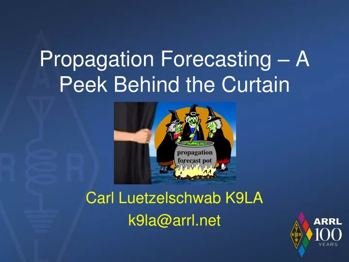
1. Propagation Forecasting – A Peek Behind the Curtain Carl Luetzelschwab K9LA k9la@arrl.net propagation forecast pot

2. Contrary to popular belief, propagation forecasting is not solely an art – there is science involved. Honest!

3. Who Is K9LA? Licensed in October 1961 as WN9AVT, K9LA in 1977 Enjoy propagation, DXing, contesting, antennas and vintage equipment • Interested in propagation since my college days • MSEE project about group delay in the ionosphere • Began doing predictions using the manual method (before PCs) • Used worldwide MUF maps, great circle path maps, control points • Great way to acquire a fundamental understanding of the process • Visit http://k9la.us for solar and propagation articles

4. Propagation Predictions Propagation predictions (alternatively, propagation forecasts) nowadays refer to using VOACAP or W6ELProp or your favorite software to determine the times and frequencies that will allow you to work a specific target This usually gives you a bunch of data For an individual trying to increase DXCC or WAZ totals, this is adequate But for a contest effort or a DXpedition team, I believe there’s more work to do in terms of ‘propagation’ Icall this‘propagation planning’

5. Common Ground and Agenda Regardless of what you do with the predictions, there is common ground – the common ground is the fact that the model of the ionosphere is a monthly median model Our agenda will thus be: Quick history and development of the model of the ionosphere How to interpret the results (MUF and signal strength) Predictions for an individual Propagation planning for contests Propagation planning for DXpeditions Cycle 24 Update

6. The Need for a Model After WWII it became apparent that it was important to be able to be on the right frequency at the right time to communicate with a desired location A model of the ionosphere was needed Ionosondes used to collect data Swept-frequency radar that looks straight up Data initially was for 1954-1958 Included solar min and solar max More data added over the years

7. Ionosonde Measurements An ionosonde gives us the critical frequencies and virtual heights of the ionospheric regions The data from the ionosonde also gives us the electron density profile (after some math) daytime data fxF2 foF2 foF1 foE electron density profile

8. Scientists Began Their Work We can predict oblique propagation from critical frequencies and heights using spherical geometry Many years of solar data and worldwide ionosonde data collected The task of the propagation prediction developers was to determine the correlation between solar data and ionosonde data It would have been nice to find a good correlation between what the ionosphere was doing on a given day and what the Sun was doing on the same day ionosonde data solar data ???

9. But That Didn’t Happen zero sunspots constant 10.7 cm flux pretty low A indices • Low of 11.6 MHz on August 14 • High of 21.5 MHz on August 16 • No correlation to daily SF and A • Three factors determine ionization • Solar radiation (3% of total daytime day-to-day std dev variation) • Geomagnetic field activity (13%) • Events in lower atmosphere couple up to ionosphere (15%)

10. Now What? Daily correlation not good - the developers were forced to come up with a statistical model over a month’s time frame monthly median correlation Monthly median correlation good – smoothed solar flux (or smoothed sunspot number) and monthly median parameters daily correlation

11. Interpreting MUF and Sig Str Our model of the ionosphere was developed to use a smoothed solar index Smoothed 10.7 cm solar flux or smoothed sunspot number equally good as there is an extremely high correlation between the two Our model of the ionosphere was developed to give monthly median MUF and monthly median signal strength Median implies 50% probability Using a daily solar index will give results that could be off by a band or two and off by many S-units

12. Example of Median After inputting a smoothed solar index, your favorite software says the MUF is 19.6 MHz and the signal strength is S7 during a specific month at a specific time On half the days of the month, the MUF will be at least 19.6 MHz On any given day during the month the MUF could be up to about 35% lower to about 25% higher On half the days of the month, the sig str will be at least S7 On any given day during the month the sig str could be several S-units lower to about an S-unit higher Unfortunately, trying to identify which days are ‘good’ and which days are ‘bad’ is tough For details on downloading VOACAP or W6ELProp and using them and interpreting the results, visit http://k9la.us

13. Real-Time Assessment For a real-time assessment of propagation, use the IARU/NCDXF beacons on 20m, 17m, 15m, 12m and 10m to give a picture of worldwide propagation http://www.ncdxf.org/pages/beacons.html Use Faros beacon software to monitor the beacons to study propagation http://dxatlas.com/faros Example on the next slide

14. Faros Results After calibration of the delays, can identify short path and long path Measures signal-to-noise ratio Can compare to propagation predictions from K2MO study Might see unusual openings, drop-outs due to geomagnetic field activity and non-great circle paths

15. Tips about: Predictions for individuals Propagation planning for contests Propagation planning for DXpeditions

16. K9LA to ZF October Fall 2014 1 kW 12 dBi antennas Req SNR = 13 dB in 3 kHz (90% voice intelligibility) 13.0 22.3 14.2 18.1 21.2 24.9 28.4 0.0 0.0 0.0 0.0 0.0 0.0 FREQ 1F2 1F2 1F2 1F2 1F2 1F2 - - - - - - MODE 9.2 4.8 5.3 6.8 10.3 10.3 - - - - - - TANGLE 8.6 8.4 8.4 8.5 8.6 8.6 - - - - - - DELAY 327 224 235 270 352 352 - - - - - - V HITE 0.50 0.99 0.91 0.63 0.20 0.02 - - - - - - MUFday 121 113 113 116 137 166 - - - - - - LOSS 33 37 37 36 16 -12 - - - - - - DBU -89 -82 -83 -85 -107 -136 - - - - - - S DBW -174 -168 -171 -173 -175 -177 - - - - - - N DBW 85 86 88 88 68 40 - - - - - - SNR -10 -26 -26 -20 6 34 - - - - - - RPWRG 0.96 1.00 1.00 0.99 0.84 0.35 - - - - - - REL 0.00 0.00 0.00 0.00 0.00 0.00 - - - - - - MPROB 0.59 0.91 0.90 0.76 0.43 0.16 - - - - - - S PRB 25.0 8.4 9.7 17.9 25.0 25.0 - - - - - - SIG LW 11.6 6.1 4.8 7.8 21.4 25.0 - - - - - - SIG UP 26.8 12.5 13.6 20.3 26.8 26.8 - - - - - - SNR LW 12.9 8.0 7.4 9.7 22.1 25.6 - - - - - - SNR UP 12.0 12.0 12.0 12.0 12.0 12.0 - - - - - - TGAIN 12.0 12.0 12.0 12.0 12.0 12.0 - - - - - - RGAIN 58 74 74 68 42 14 - - - - - - SNRxx VOACAP results

17. What Is the Best Band? We have two probabilities Probability that MUF is high enough Probability that SNR is high enough Multiply them together to get the joint probability (NM7M SK called this DX feasibility) that the MUF and the SNR are simultaneously high enough You can also do this with ‘time’ as an additional variable to identify ‘what band at what time’ is best median UTC MUF 20m 17m 15m 12m 10m 13.0 22.3 14.2 18.1 21.2 24.9 28.4 0.50 0.99 0.91 0.63 0.20 0.02 MUFday (prob that MUF is at each band) -89 -82 -83 -85 -107 -136 S DBW (in dB above 1W – add 30 for dBm) 85 86 88 88 68 40 SNR (predicted median SNR) 0.96 1.00 1.00 0.99 0.84 0.35 REL (prob that SNR > requirement)

18. QRP Considerations Fighting a pile-up with QRP can be tough Operator skill and antennas play an important role Another technique is to identify unusual openings When most others will be in bed Of course the station you’re trying to work must be aware of these unusual openings, too!

19. Propagation Planning for Contests K1TO, K9MK, W5ASP and I did a Multi-Single contest effort from ZF in CQ WW CW in 1997 One ‘run’ station – work anybody One ‘multiplier’ station – only work new multipliers After the contest I wondered if there was a way to use propagation predictions to tell the best band for the run station to be on for each hour of the contest Using the joint probability concept described earlier, I compared our actual ZF band changes to the band changes recommended by VOACAP Only needed to run predictions to NA, EU, JA

20. VOACAP vs ZF1A Decent agreement – use as a guideline Method is useful if you are not familiar with propagation from your contest location Experienced contesters likely do not need much help

21. Contesting Tips Know the contest Which QSOs are most important to maximize your score Run predictions based on the above You don’t have to necessarily run predictions to the world Be flexible The ionosphere is dynamic Most of the time one band above or below is adequate

22. Contesting Tips – con’t Get the big picture Sunspots, 10.7 cm solar flux, A index Great circle map centered on your location Headings, high latitude paths and distances from DXAID V4.5 (old DOS program)

23. Contesting Tips – con’t Understand disturbances to propagation • Geomagnetic storms • More than likely, lower worldwide MUFs at mid/high latitudes • Possible higher worldwide MUFs at low latitudes • Auroral-E propagation • VHF propagation at high latitudes • Solar radiation storms • Increased absorption in polar cap • Radio blackouts • Increased absorption on dayside of Earth

24. Propagation Planning for DXpeditions If you are the DXpedition, determine your goal Low bands, high bands or both Know where we are in a solar cycle In general, high bands best at max, low bands at min Run predictions for potential months Which are best for goals?

25. Propagation Planning for DXpeditions – con’t Know geomagnetic activity by month Least number of days with Ap < 7 around equinoxes

26. Propagation Planning for DXpeditions – con’t Know impact of ‘daylight’ wedge on 160m Triangular area in which QSOs are likely impossible from DX Atlas FT5ZM, Jan-Feb, 2014

27. Propagation Planning for DXpeditions – con’t Have a plan for thunderstorm activity Use maps of thunderstorm activity Use antennas with directivity on lower bands to set null Higher bands not affected as much from Handbook of Geophysics, USAF, 1960

28. DXpedition Tips As in propagation planning for contests, get the big picture http://www.solen.info/solar/

29. DXpedition Tips Try mitigation for disturbances to propagation Move down in frequency for geomagnetic field activity Try long path if PCA affecting polar cap via short path Move up in frequency for radio blackout

30. Summary Ionosphere varies significantly on a day-to-day basis Not well correlated to a daily solar index Explains why you see comments like “the flux was high but the higher bands were not good” Our predictions are statistical in nature over a month’s time frame Use MUF and sig str probabilities to identify best band/time In general we want a high solar flux and a low K index 6m F2 requires an extremely high solar flux for an extended period Understand disturbances to propagation and mitigation In addition to running predictions, look at: The big picture (sunspots, 10.7 cm flux, A index) Great circle paths Thunderstorms 160m ‘daylight wedge’ issue Be flexible

31. Cycle 24 Update First peak in early 2012 Second peak around early 2014 Higher bands should still be good this fall / winter