Control Systems for Robots
Control Systems for Robots. Prof. Robert Marmelstein CPSC 527 – Robotics Spring 2010. Introduction to Robot Control. We want robots to do things that might otherwise be done by intelligent, physical beings


Control Systems for Robots
E N D
Presentation Transcript
Control Systems for Robots Prof. Robert Marmelstein CPSC 527 – Robotics Spring 2010
Introduction to Robot Control • We want robots to do things that might otherwise be done by intelligent, physical beings • Biological nervous systems are often thought of as control systems for living organisms • To control a robot in this manner, we need to: • Define the state of the robot • Sense the state of the robot • Compare the state of the robot to a desired state • Decide what actions need to be taken to achieve the desired state and issue the associated commands • Translate those command into physical action • Measure the effect of those physical actions
Assumed vs. Actual Robot State Description • Physical States: • Position • Orientation (pose) • Velocity • Acceleration • Sensor states • Actuator States • Internal States: • Plans • Tasks • Behaviors
Control Engineering • Control engineering is the application of mathematical techniques to the design of algorithms and devices to control processes or pieces of machinery. • It almost always requires a model of the entity that is being controlled • If a system can be modeled by a set of linear differential equations there are well understood techniques for getting exact analytical solutions, and so designing controllers so that the output of the system is the required one
Example: Forced Spring • A forced spring can be modeled by a linear differential equation
Real-World Systems • Unfortunately, most real-world systems are non-linear in nature • Example: Pendulum • In these cases, the nonlinear system is often approximated by a linear system • For the Pendulum, assume sin() ≈ , which yields:
Control System Components • Target Value – The desired operating point of the overall system, which is speed. • Measured Value – The actual operating point of the system. It is affected by external factors such as hills, and internal factors such as the amount of fuel delivered to the engine. • Difference Value – This is the difference between the target value and the measured value. Translates into feedback. • Control Input – This is the main adjusting point of the control system. The amount of fuel delivered to the engine is the primary control input to the cruise control • Control Algorithm – Determines how to best regulate the control input to make the difference value as close to zero as possible. It does this by periodically looking at the difference value and adjusting the control input
Feedback: continuous monitoring of the sensors and reacting to their changes. Feedback control = self-regulation Two kinds of feedback: positive and negative Negative feedback acts to regulate the state/output of the system e.g., if too high, turn down, if too low, turn up thermostats, toilets, bodies, robots... Positive feedback acts to amplify the state/output of the system e.g., the more there is, the more is added lynch mobs, stock market, ant trails... Often results in system instability Feedback Defined
Open Loop Controller • The Open Loop Controller (OLC) is the simplest kind • The controller sends an input signal to the plant • It does not compensate for disturbances that occur after the control stage • Actual effects are assumed – not measured • No feedback to match actual to intended
Open Loop Controller (cont.) • The OLC is commonly used for behavior-based systems • If a trigger condition is met , then the behavior is activated • Behavior is performed until the condition is no longer met • If the condition is not met, the (assumedly) some other behavior is activated • You would likely use an OLC if you have no way of measuring your operating point (e.g., the value you are trying to control)
Problem with Open Loop Controllers • The effectiveness of OLCs are very context dependent • The amount of force that is applied has different effects dependent on the surface type
Closed Loop Controller • In Closed-loop control, the output is sensed and compared with the reference. The resulting error signal is fed back to the controller [feedback]. • Components: • Reference – Desired State • Controller – Issues Commands • Plant – Actuator
Closed Loop Controller (cont.) • [Negative] Feedback keeps the operation of the system smooth and stable • Closed Loop Controller issues: • How quickly will the system respond to error? • How long will it take the system to reach equilibrium? • What, if any, residual error will remain? • Under what conditions will the system become unstable?
Output Input Error Computation (Brain) Actuator Control (Auto Pedals) Velocity (Engine Power) + - Actual Position Desired Position Velocity Sensing (Eyes) Time Velocity Velocity decreases as the car gets closer to the desired position Example of a Closed Loop Controller
temp > target OFF ON temp < target Bang-Bang Controller (BBC) • The simplest type of closed-loop controller is the Bang-Bang controller. It typically consists of two states and a target value • The BBC typically monitors one item (quantity) of interest—its job is to keep that quantity at a certain target value • If the quantity is too high or low (vs. the target) the BBC compensates to change it • The system continually transitions between states, often abruptly
Taking the Edge off Bang-Bang Control with Hysteresis • Hysteresis provides a sort of "guard band" around the desired set point of the system. • In other words, when the temperature goes above (or below) the desired control point, there is a margin which needs to be exceeded before compensation is applied • The result a lag which causes the system to run much smoother, avoiding the jerkiness of a purely Bang-Bang controller
Leveraging Hysteresis Use of temperature dead zone to induce hysteresis Single Threshold System (no hysteresis)
JLJ Text – Fig 2.5 Closed Loop Controller Issues High Gain – Unstable Low Gain – Sluggish
Proportional Integral Derivative (PID) Controller • Closed loop controllers that only use proportional control can easily become unstable if the gain is too high or sluggish if the gain is set too low • PID controllers help solve this problem • It use the measured error compute an input to the Plant based on three distinct controls: Proportional, Integral and Derivative (see right) • Proportional control – Computed based on the actual error (times a gain factor). Thus, The larger the error, the bigger correction the control will make • Serves to control response time to error • For high gains or large errors, tends to overshoot and oscillate the desired output • There is typically a steady state error that cannot be corrected
Proportional Integral Derivative (PID) Controller • Integral control – Reduces steady-state error by adding (integrating) the actual errors over time. • Once the error reaches a predetermined threshold, the controller will compensates • Too little can result in undershoot; too much can result in overshoot • Derivative (D) control – Computed based of difference between current and previous error. Thus, the output of this control is proportional to the change in error • Prevents oscillations due to overshoot • Reduced settling time by giving a better dynamical response • Generally, this control has a positive effect
PID Controller (cont.) • The tunable factors are: • Kp – Proportional Gain factor • KI – Integral Gain Factor • KD – Differential Gain Factor • These factors are cross-coupled, so the performance of the system cannot be optimized by tuning each factor independently • Some systems can be engineered without all three PID components • The P components is always required, but P controllers alone can result in instability • PI is not accurate but converges quickly • PD converges relatively quickly reducing oscillations as it approaches the goal. • PID accurately maintains a position, but isn’t very fast.
Helpful PID Terms • Gain(s) --The parameter(s) that determine the magnitude of the system’s response. • Gain values determine whether or not the system stabilizes or fluctuates. • Finding effective gains is a trial and error process, requiring testing and recalibration. • Proportional Gain – When the value of the gain is proportional to the error. • Damping – The process of systematically decreasing a system’s fluctuations • A system is damped if it does not oscillate out of control. • Generally, the gains have to be adjusted for a system to be damped • Steady State Error – The amount of error that remains after the system has reached equilibrium
PID Controller (cont.) • KP – Proportional Gain • KI – Integral Gain • KD – Derivative Gain
PID Controller Response Curve Controlled variable Overshoot Steady state error % Reference Transient State Steady State Time Settling time
PID Response Curve (cont.) • Rise Time (Tr) – The time for the plant output y to rise beyond 90% of the desired level for the first time • Overshoot – How much the peak level is higher than the steady state, normalized against the steady state • The time required for the output to reach its maximum level is called the Peak Time (Tp) • Settling Time (Ts) – The time it takes for the system to converge to its steady state • Transient State – The period from the detection of error until its approximate correction, resulting in the steady state • Steady-state Error – The difference between the steady-state output and the desired output.
KP KI KD Effect of Increasing PID Factors NT: No trend
KP = 20 KP = 200 KP = 500 Control Performance – Proportional Control Source: CUNY – Dr. Jizhong Xiao KP = 50
KI = 200 KI = 50 Control Performance – Integral Control(KP = 100) Source: CUNY – Dr. Jizhong Xiao
KD = 2 KD = 5 KD = 20 KD = 10 Control Performance – Derivative Control(KP = 100, KI =200) Source: CUNY – Dr. Jizhong Xiao
Optimizing Performance • PID Tuning – By Hand • Boost Kp until it oscillates • Boost KD to stop oscillation, back off Kp by 10% • Dial in KI to Hold position or velocity smooth • Trial and error • PID tuning – By Design • Zeigler-Nichols Method (next slide) • Other: • Work to minimize environmental interference and sensor error (two are typically coupled) • Smart design helps too
Zeigler-Nichols Tuning Rule for PID Controllers Yields ~25% overshoot and good settling time
Why Care about the PID Controller? • Because PID Controllers are everywhere! • Due to its simplicity and excellent if not optimal performance in many applications, PID controllers are used in more than 95% of closed-loop industrial processes. • It can be tuned by operators without extensive background in Controls, unlike many other modern controllers that are much more complex but often provide only marginal improvement. • In fact, most PID controllers are tuned on-site. • The lengthy calculations for an initial guess of PID parameters can often be circumvented if we know a few useful tuning rules. This is especially useful when the system is unknown
Non-Linear Control • Linear controllers are generally valid only over small operational ranges. • Hard non-linearity cannot even be approximated by linear systems. • Model uncertainties can sometime be tolerated by the addition of non-linear terms. • Non-linear systems often have multiple equilibrium points, plus periodic, or chaotic attractors. • In these systems, small disturbances (even noise) can induce radically different behaviors.
Control System Non-Linearity Issues • Saturation – Occurs when the input signal to a certain device exceeds the ability of the device to process it • Input – sensors • Output – motors • For output, saturation means that the required compensation can no longer be applied to the control system • In general, it is good practice to limit the signal to the saturation value in software • When an input reaches the saturation point, it no longer provides a reliable estimate of the real world
Non-Linearity Issues (cont.) • Backlash – Term describing actuator hesitation and overshoot caused by small gaps between motor gears • Can result in small, but unnecessary, oscillations of the actuator position • Dead Zone – Because the sensitivity of actuators is limited, not every non-zero input will result in action. The Dead Zone is the +/- region above a zero (0) input that will result in no actuator movement.
Self-Balancing Robot Lab • Problem – Create a PID controller that will keep an NXT robot balanced on two wheels • Use a light sensor to determine balance: • Light diminishes as it tilts backward • Light gets stronger as it tilts forward • Collect reference value when the robot is perfectly balanced • PID controller will use the light sensor data to compute the compensation for the motors (plant) • Move backward if tilting back • Move forward if tilting forward
Light Sensor Self-Balancing Robot (Pics)
[Simplified] PID Controller Algorithm // Get Balance Reading for Light Sensor midVal = Sensor_Read(LS_Port); // Now Compute Power (PID) Value for Balancing Robot while (true) { lightVal = Sensor_Read(LS_Port); error = lightVal – midVal; diffErr = error – prevError; intErr = intErr + error; pVal = kp * error; iVal = (ki*intErr)*dampFactor; dVal = kd*diffErr; prevErr = error; power = (pVal+iVal+dVal)*scale; MotorFWD(motorPorts, power); }
Other Material • PID Controller for Dead Reckoning • CMU PID Tutorial • DePaul Self-Balancing Robots – Trials and Tribulations