Download
1 / 41
410 likes | 598 Vues
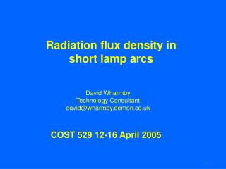
Radiation flux density in short lamp arcs. David Wharmby Technology Consultant david@wharmby.demon.co.uk. COST 529 12-16 April 2005. Outline. Why is radiation flux density (RFD) important? Line-of-sight radiation transport Optical depth Absorption coefficient Radiation flux density

E N D
Radiation flux density in short lamp arcs David Wharmby Technology Consultant david@wharmby.demon.co.uk COST 529 12-16 April 2005
Outline • Why is radiation flux density (RFD) important? • Line-of-sight radiation transport • Optical depth • Absorption coefficient • Radiation flux density • RFD in cylindrical geometry • Jones and Mottram net emission coefficient • Calculation of RFD in arbitrary geometry • Galvez’ method • Summary
Ttop = 1305K gas temperature velocity Tbottom = 1255K Tmin = 1325K Tmax = 9095K outside wall temperature Compact arcs need models for development Short arcs have strong flows, no symmetry, dominant electrode effects Time-dependence models are needed Materials are very highly stressed ~mm Source Miguel Galvez, LS10 Toulouse, 2004
W m-3 power in radiation conduction Compact 3D arc models • 50% of power may escape as radiation • High pressures mean that most of spectrum is at medium optical depth • But . . .LTE is usually OK, thankfully • Chemistry, conduction, convection and radiation must be included • Short arcs have radial and longitudinal temperature gradients, non-uniform E field • Steady state energy balance • all terms depend on temperature • solution gives the temperature field • Satisfactory treatment of radiation flux density vector FR (W m-2) is critical because radiation is so dominant Source M. Galvez, paper P-160 LS10 Toulouse, 2004
Role of radiation • E field accelerates electrons • electrons collisions produce excited states • emitted photons may escape or may be absorbed • absorption determines excited state densities • photons can travel throughout the plasma & affect excited state densities elsewhere • non-linear & non-local system • electron and excited state densities depend exponentially on T • absorption and emission processes depend very strongly on frequency • absorption depends on emission from rest of plasma Radiation transport requires massive computer resources Most approaches are unsatisfactory for short HID lamps
Il(s) s u s so r s Line of sight radiation transport • Spectral intensity (spectral radiance) of ray direction u at position rin the plasma (W m-2 sr-1 nm-1) • LTE (& Kirchhoff), no scattering, no incoming radiation • Only data needed is local value of k(l,T) • Total intensity in just one direction needs triple integration over s, ,l plasma Planck optical depth absorption coefficient
Example calculation Across diameter 100 torr Na plasma, parabolic profile 4200K-1500K, Stark & resonance broadening • SR intensities are a guide to maximum temperature • independent of oscillator strength, number density • slightly dependent of T(r) • SR dips can give some information about T(r)
Is plasma optically thin? • Information needed for experiment and model • Measurement of transmittance is unreliable in lamps • t>0.95 (say) • Better guide • compare measured spectral radiance with line-of-sight radiation transport calculation using assumed temperature distribution • At given l plasma is thin when • measured spectral radiance << Planck radiance at highest T • For energy balance calculation • radiation that is neither thick nor thin affects temperature profile • needs full RFD calculation. Source Griem “Plasma Spectroscopy”, 1964
How do we know that a plasma is optically thin? • Make spectral radiance measurement • Calculate [radiance/BB radiance] at Tmax, assuming T(r)
How do we know that a plasma is optically thin? • Make spectral radiance measurement • Calculate ratio radiance/BB radiance at Tmax, assuming T(r) • Calculate transmittance t = exp(-t)
How do we know that a plasma is optically thin? • Make spectral radiance measurement • Calculate ratio radiance/BB radiance at Tmax, assuming T(r) • Calculate transmittance t = exp(-t) • Where is t > 0.95
Absorption coefficient k(l,T) data example • Example • High pressure Hg at 8000K • Absorption from • lines: resonance, van der Waals & Stark • e-a and e-i Brems. • e-i recombination • molecular • Omission of molecular wing of lines gives imperfect line profile Source Lawler, J. Phys. D: Appl. Phys. 37, 1532-6, 2004 (e-a data for Hg) Hartel, Schoepp & Hess, J. App. Phys 85, 7076-7088, 1999 (line broadening)
9.0 6 3,1D 1S0 8.5 365 group 8.0 313 group 546 G 436 405 297 E F D B A 185 X ? Molecular absorption • Green transitions give absorption in UV 254nm resonance line • Blue transitions affect extreme wing profile of non-resonance lines • Upper levels are completely unknown • Generally bb, ff, fb and bf emission from molecules will be important 254 Source A Gallagher in “Excimer Lasers”
relative intensity % 100 80 60 40 20 0 530 534 538 542 wavelength (nm) Molecular effects in the wing of the Tl line Measurements of Tl resonance line broadened by Tl and Hg Note strongly curtailed red wing Time dependent spectra on 50Hz operation
Il(r,u2) plasma FRl(r) Il(r,u1) r Il(r,u3) Il(r,u4) Radiation flux density (RFD) • Integrate intensity (vectorially) passing through area at r in directions u • Two more integrations over q and f • This vector is radiation powerFRl through unit area at r (W m-2 nm-1) • Total RFD FR(W m-2) needs 5th integration over l • For a uniform element, div(FR) (W m-3) gives radiation power (W m-3) in element for calculation of energy balance • net emission coefficient div(FR) = 4peN • difference between emission and absorption in element of plasma
Treating radiation complexity – in order of increasing computer time Remember RFD must be evaluated many times during energy balance • Ignore it by unphysical approximations • t >>1 (diffusion) • t<<1 (optically thin) • Reduce complexity of RFD integral using symmetry • e.g cylindrical • Find a realistic way to express eN as a local quantity • Find ways to pre-tabulate some of the integral • Sevast’yanenko (pre-tabulate integration over l) • Galvez (pre-tabulate geometry) • Use Monte Carlo methods • Full-blooded numerical integration
Treating radiation complexity – in order of increasing computer time Remember RFD must be evaluated many times during energy balance often hopeless • Ignore it by unphysical approximations • t >>1 (diffusion) • t<<1 (optically thin) • Reduce complexity of RFD integral using symmetry • e.g cylindrical • Find a realistic way to express eN as a local quantity • Find ways to pre-tabulate some of the integral • Sevast’yanenko (pre-tabulate integration over l) • Galvez (pre-tabulate geometry) • Use Monte Carlo methods • Full-blooded numerical integration
Treating radiation complexity – in order of increasing computer time Remember RFD must be evaluated many times during energy balance often hopeless • Ignore it by unphysical approximations • t >>1 (diffusion) • t<<1 (optically thin) • Reduce complexity of RFD integral using symmetry • e.g cylindrical • Find a realistic way to express eN as a local quantity • Find ways to pre-tabulate some of the integral • Sevast’yanenko (pre-tabulate integration over l) • Galvez (pre-tabulate geometry) • Use Monte Carlo methods • Full-blooded numerical integration many examples – Lowke, TUe
Treating radiation complexity – in order of increasing computer time Remember RFD must be evaluated many times during energy balance often hopeless • Ignore it by unphysical approximations • t >>1 (diffusion) • t<<1 (optically thin) • Reduce complexity of RFD integral using symmetry • e.g cylindrical • Find a realistic way to express eN as a local quantity • Find ways to pre-tabulate some of the integral • Sevast’yanenko (pre-tabulate integration over l) • Galvez (pre-tabulate geometry) • Use Monte Carlo methods • Full-blooded numerical integration many examples – Lowke, TUe Jones & Mottram?
Treating radiation complexity – in order of increasing computer time Remember RFD must be evaluated many times during energy balance often hopeless • Ignore it by unphysical approximations • t >>1 (diffusion) • t<<1 (optically thin) • Reduce complexity of RFD integral using symmetry • e.g cylindrical • Find a realistic way to express eN as a local quantity • Find ways to pre-tabulate some of the RFD integral • Sevast’yanenko (pre-tabulate integration over l) • Galvez (pre-tabulate geometry) • Use Monte Carlo methods • Full-blooded numerical integration many examples – Lowke, TUe Jones & Mottram? control of approx?
Treating radiation complexity – in order of increasing computer time Remember RFD must be evaluated many times during energy balance often hopeless • Ignore it by unphysical approximations • t >>1 (diffusion) • t<<1 (optically thin) • Reduce complexity of RFD integral using symmetry • e.g cylindrical • Find a realistic way to express eN as a local quantity • Find ways to pre-tabulate some of the integral • Sevast’yanenko (pre-tabulate integration over l) • Galvez (pre-tabulate geometry) • Use Monte Carlo methods • Full-blooded numerical integration many examples – Lowke, TUe Jones & Mottram? control of approx? will examine in detail
Treating radiation complexity – in order of increasing computer time Remember RFD must be evaluated many times during energy balance often hopeless • Ignore it by unphysical approximations • t >>1 (diffusion) • t<<1 (optically thin) • Reduce complexity of RFD integral using symmetry • e.g cylindrical • Find a realistic way to express eN as a local quantity • Find ways to pre-tabulate some of the integral • Sevast’yanenko (pre-tabulate integration over l) • Galvez (pre-tabulate geometry) • Use Monte Carlo methods • Full-blooded numerical integration many examples - Lowke Jones & Mottram? control of approx? will examine in detail useful for checking out of sight
wall Infinite cylindrical geometry • treated by Lowke for Na arcs • shows contribution from various rays to RFD in blue element q s(f) f r J J Lowke JQRST 9, 839-854, 1969
wall u q s(f) f r Infinite cylindrical geometry • shows contribution at r to RFD from ray in direction u • reduce evaluation of to 4 integrations by projecting q variation onto horizontal plane using pre-tabulated function G1(t(s(f)) • FRonly has a radial component Sodium arc Jones & Mottram FR after Lowke (1969) eN = (1/4p)div(FR) J J Lowke JQRST 9, 839-854, 1969
Jones and Mottram - eN as an approximate local function • Guess temperature to start to energy balance and calculate RFD FR exactly • Calculate eN(r) from div FR • Represent eN(r) as a function (T)- Emission part depends on depends on upper state number density- Absorption part depends on FR and lower state number density • Use eNfit to represent radiationuntil energy balance converges • Recalculate eNfit • Converge energy balance again For HPS in cylindrical geometry requires only 3 RFD evaluations Jones BF & Mottram DAJ J. Phys. D: Appl. Phys. 14, 1183-94, 1981
Jones and Mottram - eNfit as an approximate local function • Makes eN seem local as long as conditions do not change too much • The closer the arc temperature profile is to the guessed profile used to calculate eNfit, the more rapid the solution of energy balance • Particularly applicable to calculating effect of • a sequence of changes of pressure or power • time-dependent solutions of energy balance because from previous input values can be used • Can this be used in 3D??? • do full RFD calculation using Galvez or other method • fit eNfit(T(u), P, FR) to FRone or more directions u This could be a powerful aid but needs to be tested
Radiation flux in asymmetric 3D plasma temperature contours 6 5 A 4 1 3 2 • Green cell A receives radiation from all other cells(e.g. n = 1 . .6) • Amount of radiation from cell n is k(l,Tn) Bl(Tn) • Absorption at A dependsk(l,TA) • These depend on local values of temperature • The heavy computation occurs because the spectrum emitted cell n is selectively absorbed in the path to A
wall wall Galvez method – geometrical precalculation • 2D picture of 3D process, showing finite volumes in calculation mesh • From a starting cell (green) take rays to other parts of the plasma
wall wall Galvez method – geometrical precalculation • 2D picture of 3D process, showing finite volumes in calculation mesh • From a starting cell (green) take rays to other parts of the plasma
wall wall Galvez method – geometrical precalculation • 2D picture of 3D process, showing finite volumes in calculation mesh • From a starting cell (green) take rays to other parts of the plasma
wall wall Galvez method – geometrical precalculation • 2D picture of 3D process, showing finite volumes (FV) in calculation mesh • From a starting cell (red) take rays to other parts of the plasma • For each ray tabulate • which FV is emitting ray • which FV the ray crosses • Distance traversed in each FV • Which FV is the exit volume geometry only!
How many rays are needed? • FV mesh • Rays emitted from a single cell chosen at random • Let cell emits N rays isotropically • N increased until the rays visit at least 95% of the cells • N used by Galvez is typically 100 • So solid angle element for each ray – 4p/N =4p/100 • Repeats checks using other FV for emission confirm 100 is about enough for a good representation of the radiation field
1 k = 0 2 3 4 5 6 7 8 9 j = 0 ray 3 1 2 3 wall 4 5 6 7 8 9 Pre-tabulate following For each ray in from each start cell Start cell s(j,k) s(4,3) Ray number r 3 Cells visited n(j,k) n(3,4) n(3,5) n(2,6) n(2,7) n(1,7) n(1,8) n(1,9) n(0,9) Distance in cell d(j,k) d(3,4) d(3,5) d(2,6) d(2,7) d(1,7) d(1,8) d(1,9) d(0,9) Exit cell e(j,k) e(0,9) Geometrically complicated integral for t then becomes a simple sum based on pre-tabulated geometry & absorption coefficients
Inner Wall Temperature Distribution Molten salts Molten salts Molten salts Molten salts Inner Wall Inner Wall Inner Wall Inner Wall Temperature Distribution Temperature Distribution Temperature Distribution Temperature Distribution Results Inner Wall Temperature Distribution • Galvez at LS10 gave an example of a MH short arc energy balance calculation with • 7400 finite volumes • 100 rays per finite volume • 19000 wavelengths • Used in design study of ceramic metal halide lamps • calculates inner wall temperature • bulge shape avoids corrosion at corners of cylinder • salt temperature is more independent of orientation – better color • bulge shape reduces mechanical stress by factor 2 Molten salts Molten salts Source S Juengst, D Lang, M Galvez, LS10 Toulouse, Paper I-14 2004
Advantages of Galvez method • Straightforward evaluation of div(FR) • In the course of energy balance FR is updated every 10 to 20 iterations • Look up tables for geometry and absorption coefficients used to calculate non-local part of integral • Spectral flux from finite volumes adjacent to wall • summed to give the spectral flux (power) distribution • this can be compared with measurements in an integrating sphere • Accuracy approaches that of full integration as number of rays N increases • As with many RFD calculations it can be parallelized • Applicable to time-dependent solutions Source M Galvez, LS10 Toulouse, Paper P-160 2004
Tmax = 9095K 3684K 3602K 3556K 3511K Tmin = 1325K 3465K Conclusions • Ray tracing precalculation of Galvez is a major advance • provides a practical solution to RFD calculations in arbitrary geometry • Computational speed means that it can be applied to arbitrary geometry with convection • Has been applied to time-dependent calculations • Example is ultra high mercury pressure video projection lamp showing gas temperature, combined with electrode sheath model Source M Galvez, LS10 Toulouse, Paper P-137 2004
The future? • Galvez method will prove to be method of choice for asymmetric arcs • Iteration will be further speeded up by Jones & Mottram semi-empirical eN approach (or something like it) • This will make radiation modelling of time-dependent short arcs practical • But • Better data on high temperature absorption coefficients will be needed, especially for bb, bf, ff molecular processes