Download
1 / 80
840 likes | 1.05k Vues
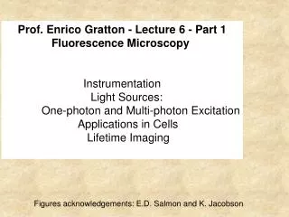
Lecture 5 FCS, Autocorrelation, PCH, Cross-correlation Enrico Gratton. Principles of Fluorescence Techniques Laboratory for Fluorescence Dynamics. Fluorescence Parameters & Methods. 1. Excitation & Emission Spectra • Local environment polarity, fluorophore concentration

E N D
Lecture 5FCS, Autocorrelation, PCH, Cross-correlationEnrico Gratton Principles of Fluorescence Techniques Laboratory for Fluorescence Dynamics
Fluorescence Parameters & Methods 1. Excitation & Emission Spectra • Local environment polarity, fluorophore concentration 2. Anisotropy & Polarization • Rotational diffusion 3. Quenching • Solvent accessibility • Character of the local environment 4. Fluorescence Lifetime • Dynamic processes (nanosecond timescale) 5. Resonance Energy Transfer • Probe-to-probe distance measurements 6. Fluorescence microscopy • localization 7. Fluorescence Correlation Spectroscopy • Translational & rotational diffusion • Concentration • Dynamics
First Application of Correlation Spectroscopy (Svedberg & Inouye, 1911) Occupancy Fluctuation Experimental data on colloidal gold particles: 120002001324123102111131125111023313332211122422122612214 2345241141311423100100421123123201111000111_2110013200000 10011000100023221002110000201001_333122000231221024011102_ 1222112231000110331110210110010103011312121010121111211_10 003221012302012121321110110023312242110001203010100221734 410101002112211444421211440132123314313011222123310121111 222412231113322132110000410432012120011322231200_253212033 233111100210022013011321113120010131432211221122323442230 321421532200202142123232043112312003314223452134110412322 220221 Collected data by counting (by visual inspection) the number of particles in the observation volume as a function of time using a “ultra microscope”
Particle Correlation *Histogram of particle counts *Poisson behavior *Autocorrelation not available in the original paper. It can be easily calculated today. They estimated the particle size to be 6 nm. Comments to this paper conclude that scattering will not be suitable to observe single molecules, but fluorescence could
Diffusion Enzymatic Activity Phase Fluctuations Conformational Dynamics Rotational Motion Protein Folding In FCS Fluctuations are in the Fluorescence Signal Example of processes that could generate fluctuations
Generating Fluctuations By Motion What is Observed? 1. The Rate of Motion 2. The Concentration of Particles 3. Changes in the Particle Fluorescence while under Observation, for example conformational transitions Observation Volume Sample Space
Approximately 1 um3 Defining Our Observation Volume: One- & Two-Photon Excitation. 2 - Photon 1 - Photon Defined by the pinhole size, wavelength, magnification and numerical aperture of the objective Defined by the wavelength and numerical aperture of the objective
1-photon Need a pinhole to define a small volume 2-photon Brad Amos MRC, Cambridge, UK
Data Treatment & Analysis Time Histogram Autocorrelation Autocorrelation Parameters: G(0) & kaction Photon Counting Histogram (PCH) PCH Parameters: <N> & e
Autocorrelation Function Factors influencing the fluorescence signal: kQ = quantum yield and detector sensitivity (how bright is our probe). This term could contain the fluctuation of the fluorescence intensity due to internal processes C(r,t) is a function of the fluorophore concentration over time. This is the term that contains the “physics” of the diffusion processes W(r) describes our observation volume
The Autocorrelation Function t3 t5 t4 t2 t1 G(0) 1/N As time (tau) approaches 0 Diffusion
Calculating the Autocorrelation Function Photon Counts time Average Fluorescence t + t t
<N> = 2 <N> = 4 The Effects of Particle Concentration on the Autocorrelation Curve
Why Is G(0) Proportional to 1/Particle Number? A Poisson distribution describes the statistics of particle occupancy fluctuations. In a Poissonian system the variance is proportional to the average number of fluctuating species:
G(0), Particle Brightness and Poisson Statistics 1 0 0 0 0 0 0 0 0 2 0 1 1 1 0 0 0 0 0 0 1 0 0 0 0 0 0 0 1 0 1 0 0 0 1 0 0 1 0 0 Time Average = 0.275 Variance = 0.256 Lets increase the particle brightness by 4x: 4 0 0 0 0 0 0 0 0 8 0 4 4 4 0 0 0 0 0 0 4 0 0 0 0 0 0 0 4 0 4 0 0 0 4 0 0 4 0 0 Average = 1.1 Variance = 4.09 0.296
Effect of Shape on the (Two-Photon) Autocorrelation Functions: For a 2-dimensional Gaussian excitation volume: 1-photon equation contains a 4, instead of 8 For a 3-dimensional Gaussian excitation volume:
Additional Equations: 3D Gaussian Confocor analysis: ... where N is the average particle number, tD is the diffusion time (related to D, tD=w2/8D, for two photon and tD=w2/4D for 1-photon excitation), and S is a shape parameter, equivalent to w/z in the previous equations. Triplet state term: ..where T is the triplet state amplitude and tT is the triplet lifetime.
Orders of magnitude (for 1 μM solution, small molecule, water) Volume Device Size(μm) Molecules Time milliliter cuvette 10000 6x10¹⁴ 104 microliter plate well 1000 6x10¹¹ 102 nanoliter microfabrication 100 6x10⁸ 1 picoliter typical cell 10 6x10⁵ 10-2 femtoliter confocal volume 1 6x10² 10-4 attoliter nanofabrication 0.1 6x10⁻¹ 10-6
The Effects of Particle Size on the Autocorrelation Curve Diffusion Constants 300 um2/s 90 um2/s 71 um2/s Slow Diffusion Fast Diffusion Stokes-Einstein Equation: and Monomer --> Dimer Only a change in D by a factor of 21/3, or 1.26
Autocorrelation Adenylate Kinase -EGFP Chimeric Protein in HeLa Cells Examples of different Hela cells transfected with AK1-EGFP Fluorescence Intensity Examples of different Hela cells transfected with AK1b -EGFP Qiao Qiao Ruan, Y. Chen, M. Glaser & W. Mantulin Dept. Biochem & Dept Physics- LFD Univ Il, USA
Autocorrelation of EGFP & Adenylate Kinase -EGFP EGFP-AK in the cytosol G(t) EGFP-AKb in the cytosol EGFPsolution EGFPcell Time (s) Normalized autocorrelation curve of EGFP in solution (•), EGFP in the cell (•), AK1-EGFP in the cell(•), AK1b-EGFP in the cytoplasm of the cell(•).
Autocorrelation of Adenylate Kinase –EGFP on the Membrane Clearly more than one diffusion time A mixture of AK1b-EGFP in the cytoplasm and membrane of the cell.
Autocorrelation Adenylate Kinaseb -EGFP Plasma Membrane Cytosol D D Diffusion constants (um2/s) of AK EGFP-AKb in the cytosol -EGFP in the cell (HeLa). At the membrane, a dual diffusion rate is calculated from FCS data. Away from the plasma membrane, single diffusion constants are found.
Multiple Species G(0)sample is no longer g/N ! Case 1: Species vary by a difference in diffusion constant, D. Autocorrelation function can be used: (2D-Gaussian Shape) !
Antibody - Hapten Interactions Binding site Binding site carb2 Digoxin: a cardiac glycoside used to treat congestive heart failure. Digoxin competes with potassium for a binding site on an enzyme, referred to as potassium-ATPase. Digoxin inhibits the Na-K ATPase pump in the myocardial cell membrane. Mouse IgG: The two heavy chains are shown in yellow and light blue. The two light chains are shown in green and dark blue..J.Harris, S.B.Larson, K.W.Hasel, A.McPherson, "Refined structure of an intact IgG2a monoclonal antibody", Biochemistry 36: 1581, (1997).
Anti-Digoxin Antibody (IgG) Binding to Digoxin-Fluorescein triplet state Digoxin-Fl•IgG (99% bound) Autocorrelation curves: Digoxin-Fl•IgG (50% Bound) Digoxin-Fl Binding titration from the autocorrelation analyses: Kd=12 nM S. Tetin, K. Swift, & , E, Matayoshi , 2003
Two Binding Site Model IgG•2Ligand-Fl + Ligand-Fl IgG + 2 Ligand-Fl IgG•Ligand-Fl 50% quenching Kd IgG•Ligand No quenching IgG•2Ligand [Ligand]=1, G(0)=1/N, Kd=1.0
Digoxin-FL Binding to IgG: G(0) Profile Y. Chen , Ph.D. Dissertation; Chen et. al., Biophys. J (2000) 79: 1074
Case 2: Species vary by a difference in brightness assuming that The quantity Go becomes the only parameter to distinguish species, but we know that: The autocorrelation function is not suitable for analysis of this kind of data without additional information. We need a different type of analysis
Sources of Non-Poissonian Noise Detector Noise Diffusing Particles in an Inhomogeneous Excitation Beam* Particle Number Fluctuations* Multiple Species* Photon Counting Histogram (PCH) Aim: To resolve species from differences in their molecular brightness Poisson Distribution: Single Species: Where p(k) is the probability of observing k photon counts
PCH Example: Differences in Brightness frequency (en=1.0) (en=2.2) (en=3.7) Increasing Brightness Photon Counts
Single Species PCH: Concentration 5.5 nM Fluorescein Fit: e = 16,000 cpsm N = 0.3 550 nM Fluorescein Fit: e = 16,000 cpsm N = 33 As particle concentration increases the PCH approaches a Poisson distribution
Photon Counting Histogram: Multispecies Binary Mixture: Molecular Brightness Concentration Snapshots of the excitation volume Intensity Time
Sample 1: fewer but brighter fluors (10 nM Rhodamine) Sample 3: The mixture Photon Counting Histogram: Multispecies Sample 2: many but dim (23 nM fluorescein at pH 6.3) The occupancy fluctuations for each specie in the mixture becomes a convolution of the individual specie histograms. The resulting histogram is then broader than expected for a single species.
Examination of a Protein Dimer with FCS: Secreted Phospholipase A2 Sanchez, S. A., Y. Chen, J. D. Mueller, E. Gratton, T. L. Hazlett. (2001) Biochemistry, 40, 6903-6911.
membrane sPLA2 Interfacial Binding sPLA2 Self-Association sPLA2 Membrane Binding Interfacial sPLA2Self-Association
Lipid Interfaces Choline Group Multibilayers (MLVs) Vesicles (SUVs, LUVs & GUVs) 12 Carbon Tail Micelles Dodecylphosphocholine (DPC) Micellar Lipid Analog (CMC = 1.1 mM)
In Solution: a Tight Dimer Fluorescein-sPLA2 Steady-State Anisotropy Fluorescence Correlation Spectroscopy [Fl-sPLA2] [Fl-sPLA2] measured predicted (by sedimentation) Time-Resolved Anisotropy: Rotational correlation time 1 = 12.8 ns (0.43) Rotational correlation time 2 = 0.50 ns (0.57) Why this large discrepancy?
In Solution: Fluorescein-sPLA2 +/- Urea 1. Autocorrelation sPLA2 G(0)=0.021 D = 72 um2/s Increasing Particles sPLA2 + 3M Urea G(0)=0.009 D = 95 um2/s 2. PCH analysis sPLA2 e = 0.6 N = 3.29 sPLA2 + 3M Urea e = 0.6 N = 8.48 Increasing Particles Adjusted for viscosity differences Change in number of particles, little change in brightness!
The Critical Question: Is sPLA2 a Dimer in the Presence of Interfacial Lipid? What Could We Expect to Find in the FCS Data? Monomer Lipid Micellar Lipid C.atrox sPLA2 Ddimer N particles (Preferred Substrate) (Poor Substrate) Upon dissociation, the mass could increase due to lipid binding. Better count the number of particles! Observing Fluorescein-labeled sPLA2
FCS on Fluorescein - sPLA2 in Buffer (RED) and with DPC Micelles ( BLUE ) 1. Autocorrelation Analysis +DPC = increase in particles sPLA2 G0 = 0.0137 D = 75 um2/s sPLA2 + 20 mM DPC G0 = 0.0069 D = 55 um2/s 2. PCH Analysis sPLA2 e= 0.41 N = 6.5 sPLA2 + 20 mM DPC e = 0.45 N = 12.2 +DPC = increase in particles
Fluorescein-sPLA2 Interaction with DPC N Ca2+ EDTA (Dmicelle=57 um2/s) D = 55-60 um2/s 12 10 (Ddimer= 75 um2/s) N D = 73 um2/s 8 • The PLA2 dimer dissociates in the presence of micelles. • Active enzyme form in a micellar system is monomeric. 6 0.01 0.1 1 10 [DPC] (mM)
+ + + + + + + + + + + + + + + + + + + + + + + + + + + + + + + + + + + + + + + + + + + + + + + + + + + + + + + + + + + + + + + + + + + + + + + + + + Schematic of sPLA2 - Dodecylphosphocholine Interactions Monomer-Lipid Association sPLA2 sPLA2-Micelle Co-Micelle
Two Channel Detection: Cross-correlation Sample Excitation Volume Beam Splitter • Increases signal to noise by isolating correlated signals. • Corrects for PMT noise Detector 1 Detector 2 Each detector observes the same particles
Removal of Detector Noise by Cross-correlation Detector 1 11.5 nM Fluorescein Detector 2 Detector after-pulsing Cross-correlation
Calculating the Cross-correlation Function Detector 1: Fi time t + t t Detector 2: Fj time
Cross-correlation Calculations One uses the same fitting functions you would use for the standard autocorrelation curves. Thus, for a 3-dimensional Gaussian excitation volume one uses: G12 is commonly usedto denote the cross-correlation and G1 and G2 for the autocorrelation of the individual detectors. Sometimes you will see Gx(0) or C(0) used for the cross-correlation.
Two-Color Cross-correlation The cross-correlation ONLY if particles are observed in both channels Sample Green filter Red filter Each detector observes particles with a particular color The cross-correlation signal: Only the green-red molecules are observed!!
Two-color Cross-correlation Equations are similar to those for the cross correlation using a simple beam splitter: Information Content Signal Correlated signal from particles having bothcolors. Autocorrelation from channel 1 on the green particles. Autocorrelation from channel 2 on the red particles.