Download
1 / 17
240 likes | 565 Vues
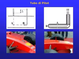
Tubo di Pitot. Tubo di Pitot. Flussi laminari e flussi turbolenti. PUNTO CRITICO IPERBOLICO. Approccio topologico : punti critici iperbolici ed ellittici, geometria frattale e strutture ad “ 8 in 8” (es.: Antonia et al. 1986, Davila & Vassilicos 2003). PUNTO CRITICO ELLITTICO. 6/ 19.

E N D
PUNTO CRITICO IPERBOLICO • Approccio topologico: punti critici iperbolici ed ellittici, geometria frattale e strutture ad “8 in 8” (es.: Antonia et al. 1986, Davila & Vassilicos 2003). PUNTO CRITICO ELLITTICO 6/ 19 C.1.1 TURBOLENZA • Turbolenza presente in molti campi dell’ingegneria(aerodinamica, diluizione di inquinanti, studio della scia a valle di un corpo in movimento, miscelazione e combustione in reattori chimici, moto dell’aria nell’apparato respiratorio e del sangue a valle di valvole cardiache, ecc.). • Turbolenza: fenomeno non totalmente compreso ma non casuale: le statistiche della separazione di coppie di particelle (~t3) sono diverse da quelle dei random walks (~t1) (Ottino 1990).
C.1.2 TURBOLENZA 2D in atmosfera VORTICE E PUNTO CRITICO ELLITTICO 7/ 19 • Turbolenza quasi-bidimensionale (Q2D): importanza teorica (semplificazione della 3D ma anche peculiarità: conservazione lagrangiana della vorticità, cascata inversa dell’energia, ecc.)e pratica(es. previsioni atmosferiche, moto delle masse d’acqua negli oceani e nell’atmosfera). GETTO 2D PUNTI CRITICI IPERBOLICI
Measurement via PTVA of the acceleration on quasi-two-dimensional turbulent-like flows controlled by multi-scale electromagnetic forces Simone Ferrari(1)(2), Lionel Rossi(2) and John Christos Vassilicos(2) (1) (2)
a b Electrodes Electrodes Magnets Tank size: 1700x1700 mm² Brine layer’s thickness: 5 mm c d 1.2. Q2D EM controlled multi-scale flows • Experimental set-up: a shallow layer of brine EM forced. • Topology and forcing time-dependency are known and controlled. • Power-law shaped energy spectrum and Richardson-like pair dispersion properties (Rossi et al., JFM 2006) in a laminar steady flow. • Experiments: constant and time-dependent forcing. Magnets’ size: 160 mm, 40 mm, 10 mm Flow visualizations with constant forcing; (a, b, c: whole field; d: SW quarter) Stirring on the SW quarter (same flow on the left) 4/ 17
Constant forcing Time-dependent forcing
3.5 Time dependent flows Mass exchange between large and medium scales is enhanced. Mass exchange between small and medium scales is enhanced. • Time dependent forcing with different frequencies, mean intensities and magnitudes, to excite different flow scales. • A further step towards fully controlled turbulent-like flows. Expected time scales of the three scales of forcing t versus current I; M160, M40 and M10 refers to the magnets’ size; the black straight line identifies the current value over which the bottom friction is no more negligible. 15/ 17
3.1 Results: measured trajectories = hyperbolic stagnation point = elliptical stagnation point large scalesmedium scalessmall scales • Trajectories are measured at all the scales of the flow (stagnation points with three different length scales). Example of measured trajectories (8 runs): on the left the whole investigation field, on the right a zoom on the SW quarter MAGNETS’ POSITION 10/ 17
3.2 Results: Eulerian fields VELOCIY: hyperbolic stagnation point; elliptical stagnation point ACCELERATION: “source”; “sink”; “spreader” The mesh has 600x600 points with a mesh’s size of 3x3 pixels (resolution 4 times higher than PIV) 11/ 17
Accelerazione Velocità Deformazione • Flusso con accelerazione locale nulla. • L’accelerazione è alta dove sia la velocità che la deformazione sono alte. Accelerazione 12a/ 17
3.3 Results: Navier-Stokes equations’ terms Viscous term Acceleration Velocity • A zoom on the SW quarter to highlight the physical coherence of the measures. • Acceleration is much larger than viscous term everywhere but at the small scales (like in turbulent flows). This allows an indirect measure of the pressure gradient over all the investigation field. Acceleration and viscous term in pixel/s2, velocity in pixel/s; 1 pixel = 0.495 mm 12b/ 17
Ñ·a u·a Stirring intensity, in s-2; 1 pixel = 0.495 mm • Experimental measure of Ñ×a over the whole investigation field. • Local maxima of Ñ×a correspond to acceleration sources, local minima of Ñ×a correspond to acceleration sinks. • Stirring is stronger where Ñ×a large and positive (Vassilicos, 2002): • the points of highest stirring are not the ones connected to the largest power input. 3.4 Results: towards efficient mixing MAGNETS’ POSITION Power input and output, in pixel2/s3; 1 pixel = 0.495 mm • The power input-output is closely related to the pressure term. • Tools to optimize the power input according to the required mixing => efficient mixing. 14/ 17