Download
1 / 42
420 likes | 529 Vues
Climate Test Bed Seminar Series 4 February 2009. Factors Limiting the Current Skill of Forecasts: Flaws in Model and Initialization. Emialia K. Jin. Center for Ocean-Land-Atmosphere studies (COLA) George Mason University (GMU). What is limiting the ENSO p redictability?. Model Flaws

E N D
Climate Test Bed Seminar Series 4 February 2009 Factors Limiting the Current Skill of Forecasts: Flaws in Model and Initialization Emialia K. Jin Center for Ocean-Land-Atmosphere studies (COLA) George Mason University (GMU)
What islimitingthe ENSO predictability? • Model Flaws • mean error, phase shift, different amplitude, and wrong seasonal cycle, etc • Flaws in the way the data is used • data assimilation and initialization,chaos within non-linear dynamics of the coupled system • Inherent limits to predictability • some times are more predictable than others, amplitude of SST anomalies with respect to ENSO phase • Gaps in the observing system
What islimitingthe ENSO predictability? • Model Flaws • mean error, phase shift, different amplitude, and wrong seasonal cycle, etc • Flaws in the way the data is used • data assimilation and initialization,chaos within non-linear dynamics of the coupled system • Inherent limits to predictability • some times are more predictable than others, amplitude of SST anomalies with respect to ENSO phase • Gaps in the observing system
Flaws in Model: Two Flavors of ENSO and Its Predictability Authors: Emilia K. Jin1, J.-S. Kug2, F.-F. Jin2, J.-J. Luo3, and T. Yamagata3 1George Mason Univ./COLA, 2University of Hawaii, 3FRCGC/JAMSTEC
Background and Objective • Conventional El Niño : “as a phenomenon in the equatorial Pacific Ocean characterized by a positive sea surface temperature departure form normal in the NINO 3.4 region greater than or equal in magnitude to 0.5C averaged over three consecutive months” (NOAA) • Different flavors of El Niño • Trans- Niño (Trenberth and Stepaniak,2001), Dateline El Niño (Larkin and Harrison 2005), El NiñoModoki (Ashok et al. 2007), Non-canonical ENSO (Guan and NIgam, 2008), Warm pool El Niño(Kug et al. 2008), etc. • : Even though there are differences, the distinctive interannual SST variation over the central Pacific which becomes more active in recent year and significantly different global impact form conventional El Niñoare common features. • The transition mechanisms and dynamical structure of two-types of El Nino are significantly different (Kug et al. 2008). • In this study, CGCM’s ability to predict the distinctive characteristics of two types of El Niño is investigated using two state-of-the-art CGCMs retrospective forecasts.
Observed Two Types of El Nino Normalized NINO3 and NINO4 SST NINO4 NINO3 Composite of SST (Contour) and Rainfall (Shaded) (1982/83, 1986/87, 1997/98) Warm-pool Cold-tongue Mixed Either NINO3 SST or NINO4 SST is greater than their standard deviation (1990/91, 1994/95, 2002/03, 2004/05) Kug et al., 2008
Observed DJF SST Anomalies Mixed Cold-tongue Warm-pool
Model and Dataset • Initial condition cases of 12 calendar months are analyzed. • As observational counterparts, OISST, CMAP rainfall, and NCEP/NCAR reanalysis data are used. Retrospective Forecast • In this study, forecast data is reconstructed with respect to lead time (monthly forecast composite). Courtesy of J.-J. Luo, T. Yamagata, and NCEP EMC
Observed DJF SST Anomalies Mixed Cold-tongue Warm-pool
Simulated SODJFM SST Anomalies Forecast lead month 1 SINTEX CFS Cold-tongue Cold-tongue Warm-pool Warm-pool Shading is for model, and contour is for observation
Simulated DJF SST Anomalies Forecast lead month 6 SINTEX CFS Cold-tongue Cold-tongue Warm-pool Warm-pool Note: loss of predictability in the Warm Pool El Nino cases Shading is for model, and contour is for observation
Composite of SST Anomalies along the Equator Forecast lead month 7 Shading is for model bias, Contour is for observed composite Note: Positive anomaly and negative bias in the Warm Pool and Cold Tongue Mixed Cold-tongue Warm-pool time CFS SINTEX time
Interannual Variability of NINO3 and NINO4 SINTEX CFS NINO3 NINO3 NINO4 NINO4 Jan Feb Mar Apr May Nov Dec Observed Jun Jul Aug Sep Oct
Scatter Diagram of Normalized DJF NINO3 vs. NINO4 SINTEX CFS Lead month 1 NINO4 Index Lead month 7 NINO3 Index
Relationship between NINO3 and NINO4 SINTEX CFS COR=0.69
Impact of Couplde Model Error on Predictability 1st mode SEOF of SST (Low frequency mode) 1st month 5th month 9th month Obs. long run SINTEX-F MAM NCEP CFS JJA Jin and Kinter, 2009 Climate Dynamics Correlation coefficients with respect to lead month Temporal correlation of PC timeseries with observation Pattern correlation of eigenvector with free long run SINTEX-F NCEP CFS SINTEX-F NCEP CFS Correlation • With increase of the lead month, the forecast ENSO mode progressively approaches to the model intrinsic mode in free coupled run and departs from the observed. Forecast lead month
Model and Dataset Free long run forecast • 1982-2004 period • 9 members • 12 calendar months ICs • 12 months lead • 202-year simulation • Analyzing last 200 years • (200-yr climatology) PRCGC SINTEX Luo et al. 2005 • 1981-2003 period • 15 members • 12 calendar months ICs • 9 months lead • 52-year simulation • Analyzing last 50 years • (50-yr climatology) NCEP CFS Saha et al. 2006 Courtesy of J.-J. Luo, T. Yamagata, and K. Pegion
Scatter Diagram of Normalized DJF NINO 3 vs. NINO 4 From free long run of two CGCMs SINTEX CFS Obs. 1950-2005 50 years 200 years NINO4 Index NINO3 Index COR=(NINO3, NINO4) 0.69 0.82 0.86 Shading: Observed; models do not capture observed behavior Model Flaw: One Flavor of El Nino
Observed Composite of Precipitation Anomalies Cold-tongue Warm-pool Obs. Forecast lead month 6 SINTEX CFS
500 hPa GPH Anomalies Cold-tongue Warm-pool Obs. Forecast lead month 6 CFS SINTEX
Summary • In two state-of-the-art CGCMs, the forecast skill of El Niño is investigated focusing on two flavors of El Niño: Warm-pool and cold-tongue. • As the lead month of forecast increases, the models fail to distinguish between two flavors of El Niño. • Both models have difficulties to reproduce the nonlinear relationship between NINO3 and NINO4 SST anomalies. • From the free long run, models tend to simulate the mixed mode of El Nino rather than warm-pool or cold-tongue El Niño. • Tropical precipitation and extratropical circulation anomalies associated with two flavors of El Niño are not captured by models.
What islimitingthe ENSO predictability? • Model Flaws • mean error, phase shift, different amplitude, and wrong seasonal cycle, etc • Flaws in the way the data is used • data assimilation and initialization,chaos within non-linear dynamics of the coupled system • Inherent limits to predictability • some times are more predictable than others, amplitude of SST anomalies with respect to ENSO phase • Gaps in the observing system
Flaws in the initialization: Impact of Ocean Initialization in CCSM3.0 Re-forecast Experiments Authors: Emilia K. Jin12, B. Kirtman23, D.-H. Min3, K. Ashok4 and H-I. Jeong4 1George Mason Univ., 2COLA, 3Univ. of Miami/RSMAS, 4APEC Climate Center
Model and Dataset • CCSM 3.0: CAM3 T85L26 + POP 1.4gx1v3 L40 • Initial condition case of November are analyzed. • As observational counterparts, OISST and CMAP rainfall are used. Retrospective Forecast Courtesy of K. Ashok and H. Jeong (APEC Climate Center), and Ben Kirtman and Dug-Hong Min (Univ. of Miami)
Ocean Initialization SST-nudged scheme MOM3 ODA 6 atm. ICs GFDL MOM3 Ocean Data Assimilation Grid interpolation to POP 1.4gx1v3 L40 APCC re-forecasts: 2-dimensional ocean initialization COLS re-forecasts: 3-dimensional ocean initialization
Root-mean-square error of NINO Indices Nov Dec Jan Feb Mar Apr May Nov Dec Jan Feb Mar Apr May Forecast lead month
Anomaly Correlation Coefficients of NINO Indices Nov Dec Jan Feb Mar Apr May Nov Dec Jan Feb Mar Apr May Forecast lead month
Temporal Correlation Coefficients of SST Anomalies DJF (1st season) MAM (2nd season)
Temporal Correlation Coefficients of SST Anomalies Differences of Correlation (APCC minus COLA)
Pattern Correlation of SST Anomalies 1st season (lead month 2-4) APCC member COLA member Pattern Correlation Coefficients (160-280E, 30S-30N) (40-160E, 30S-30N) Year
1984 SST anomalies along the Equator Forecast lead month
ACC of NINO 3.4 Index (November IC) • Colored dots denote14 CGCMs re-forecasts from DEMETER and APCC/CliPAS (Jin et al. 2008). • Tier-1 MME: 10 CGCM multi-model ensemble except NASA, UH, APCC and COLA. • Dynamic-Statistical Model: MME of modified CZ model, two statistical models and persistence • Black line denotes persistence.
RMSE of NINO 3.4 Index (Nov IC) • Colored dots denote14 CGCMs re-forecasts from DEMETER and APCC/CliPAS (Jin et al. 2008). • Tier-1 MME: 10 CGCM multi-model ensemble except NASA, UH, APCC and COLA. • Dynamic-Statistical Model: MME of modified CZ model, two statistical models and persistence • Black line denotes persistence.
Influence of Systematic Error on CFS Forecast Skill CORR. with respect to lead month based on 1st SEOF mode of SST NINO3: Warm minus Cold composite Correlation SST anomalies Forecast lead month (Hindcast composite) Correlation between 1st PCs based on observation andhindcasts at different lead times Correlation between 1st PCs based on long run and hindcasts at different lead times Observation CFS long run • Warm composite (82/83, 86/87, 91/92, 97/98) - Cold composite (84/85, 88/89, 98/99, 99/00) • Dashed lines denote composite for Hindcasts at different lead times Jin and Kinter, Climate Dynamics 2009 Model Flaw: Slow coupled dynamics of CGCM
DJF SST Climatology 1st season of Nov IC A 138-year long run of CCSM3.0 Retrospective forecasts
Composite Analysis of Nino34 Index El Nino composite Warm minus Cold composite La Nina composite • Warm composite (82/83, 86/87, 91/92, 97/98) - Cold composite (84/85, 88/89, 98/99, 99/00) • For CCSM3.0 free long run, events more than one • standard deviation of DJF NINO 3 index is selected and 32 El Niño and 24 La Niña is picked up.
DJF Correlation of SST with Precipitation Local SST NINO3.4 Re-Forecasts (Nov IC) Re-Forecasts (Nov IC) Free long run
DJF Precipitation Climatology 1st season of Nov IC A 138-year long run of CCSM3.0 Retrospective forecasts
Temporal Correlation Coefficients of Precipitation Anomalies DJF MAM
Summary • In this study, the intercomparison of long-lead coupled prediction experiments has conducted focusing on the multiple sets of retrospective forecasts with two types of initial conditions using same CCSM3.0 CGCM: 2-dimensional ocean initialization (SST nudged scheme) and 3-dimensional ocean initialization (MOM3 Ocean Data Assimilation). • Focusing on ENSO forecast, the ocean initialization of the COLA re-forecasts causes the remarkable improvement of forecast skill in spite of the large systematic errors of model. On the other hand, the APCC re-forecasts has little advantages of ocean initialization and the influence of model’s systematic errors are quite large. • These results emphasize the importance of initialization of forecast model, in particular ocean component.
Thank You ! Emilia K. Jin kjin@cola.iges.org