Download
1 / 141
1.43k likes | 1.8k Vues
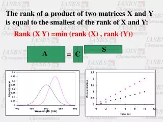
S. A. C. The rank of a product of two matrices X and Y is equal to the smallest of the rank of X and Y:. Rank (X Y) =min (rank (X) , rank (Y)). =. Eigenvectors and Eigenvalues. 0. v. R. I. R. v. = l. - l. v. For a symmetric, real matrix, R , an eigenvector v is obtained from:.

E N D
S A C The rank of a product of two matrices X and Y is equal to the smallest of the rank of X and Y: Rank (X Y) =min (rank (X) , rank (Y)) =
Eigenvectors and Eigenvalues 0 v R I R v =l -l v For a symmetric, real matrix, R, an eigenvector v is obtained from: Rv = vl l is an unknown scalar-the eigenvalue (R – lI) v= 0 Rv – vl = 0 The vector v is orthogonal to all of the row vector of matrix (R-lI) =
0.1 0.2 0.3 0.2 0.4 0.6 A= R=ATA = 0.14 0.28 0.28 0.56 0.14 0.28 0.28 0.56 0.14 0.28 0.28 0.56 v1 v2 0 0 1 0 0 1 - l v1 v2 l 0 0 l 0.14 - l 0.28 0.28 0.56 - l v1 v2 0 0 - Rv = vl (R – lI) v= 0 = = =
0.14 - l 0.28 0.28 0.56 - l = 0 (0.14 – l) (0.56 –l) – (0.28) (0.28) = 0 l2 - 0.7l = 0 l1 = 0.7 & l2=0 l (l - 0.7) = 0
v11 v21 0.14 – 0.7 0.28 0.28 0.56 – 0.7 0 0 -0.56 0.28 0.28 -0.14 v11 v21 = = -0.56 v11 + 0.28v21= 0 0.28 v11 - 0.14 v21= 0 0.4472 0.8944 Normalized vector v1 = For l1 = 0.7 v21 = 2 v11 If v11 = 1 v21= 2
v12 v22 0 0 0.14 0.28 0.28 0.56 = 0.14 v12 + 0.28 v22 = 0 0.28 v12 +0.56 v22 = 0 -0.8944 0.4472 Normalized vector v1 = For l1 = 0 v12= -2 v22 If v22 = 1 v12= -2
0.1 0.2 0.3 0.2 0.4 0.6 A= R=ATA = 0.14 0.28 0.28 0.56 -0.8944 0.4472 0.4472 0.8944 0.7 0 0 0 V = L = ∑ tr(R) = li= 0.7 + 0.0 =0.7 Rv = vl RV = VL v1v2 =0 More generally, if R (p x p) is symmetric of rank r≤p then R posses r positive eigenvalues and (p-r) zero eigenvalues
? Show that in the presence of random noise the number of non-zero eigenvalues is larger than numbers of components
Variance-Covariance Matrix … x11 – mx1 x12 – mx2 x1p – mxp … x21 – mx1 x22 – mx2 x1p – mxp X = … … … … … xnp – mxp xn2 – mx2 (xn1 – mx1) … var(x1) covar(x1x2) covar(x1xp) … covar(x2x1) var(x2) covar(x2xp) XTX = … … … … … var(xp) covar(xpx1) covar(xpx2) Column mean centered matrix
? Use anal.m file and mmcn.m file and verify that each eigenvalue of an absorbance data matrix is correlated with variance of data
Singular Value Decomposition SVD of a rectangular matrix X is a method which yield at the same time a diagnal matrix of singular values S and the two matrices of singular vectors U and V such that : X = U S VT UTU = VTV =Ir The singular vectors in U and V are identical to eigenvectors of XXT AND XTX, respectively and the singular values are equal to the positive square roots of the corresponding eigenvalues X = U S VT XT = V S UT X XT= U S VT VSUT= US2UT (X XT) U = US2
n n n n n S VT X X U n n m m m r n r S VT r r U m = If the rank of matrix X=r then; X = U S VT = s1u1v1T + … + srurvrT =
residual Reconstructed data R1 Ideal data Ideal data Noised data A A nd rd residual R2 Consider 15 sample containing 2 component with strong spectral overlapping and construct their absorbance data matrix accompany with random noise - = - = It can be shown that the reconstructed data matrix is closer to ideal data matrix
Noised data matrix, nd, with 0.005 normal distributed random noise
nf.m file for investigating the noise filtering property of svd reconstructed data
? Plot the %relative standard error as a function of number of eigenvectors
Principal Component Analysis (PCA) x11 x12 … x114 x2 … x21 x21 x214 • • • • • • • • • • • • • • x1
u11 u2 u12 • • • • u1 • … • • • • • u114 • • • • PCA
x2 x11 x12 … x114 • • • • … x21 x21 x214 • • • • • • • • • • x1
u11 u21 u2 u1 • • u12 u22 • • … … • • u114 u214 • • • • • • • •
l1 l2 s1 0.1 0.2 0.2 0.4 0.3 0.6 s2 s3 Principal Components in two Dimensions u1 = ax1 + bx2 u2 = cx1 + dx2 In principal components model new variables are found which give a clear picture of the variability of the data. This is best achieved by giving the first new variable maximum variance, the second new variable is then selected so as to be uncorrelated with the first one, and so on
0.5 1.0 1.5 0.1 0.2 0.3 u1 = 0.2 0.4 0.6 x1 = x2 = 1.0 2.0 3.0 u1 = The new variables can be uncorrelated if: ac + bd =0 Orthogonality constraint a=1 b=2 c=-1 d=0.5 var(u1)=0.25 a=2 b=4 c=-2 d=1 var(u1)=1.0