Linear Algebra
Linear Algebra. Linear algebra deals with vectors and matrices. Vectors and matrices represent collections of quantities. A single vector or matrix corresponds to many different numbers or variables. Since vectors and matrices differ by dimensionality, we shall begin with matrices.


Linear Algebra
E N D
Presentation Transcript
Linear algebra deals with vectors and matrices. Vectors and matrices represent collections of quantities. A single vector or matrix corresponds to many different numbers or variables. Since vectors and matrices differ by dimensionality, we shall begin with matrices.
A matrix is a one or two dimensional array of numbers or variables.
The collection of numbers or variables is treated as a single entity. Thus, we can perform operations on matrices and affect all of the elements within the resultant matrix.
One operation on matrices is scalar multiplication. When we multiply a matrix by a scalar we multiply every element in that matrix by that scalar. If then
Another operation on matrices is matrix addition. When we add two matrices we add them element-by-element. If then
Another operation on matrices is matrix multiplication. Multiplication is a little more complicated than addition. The product is taken by multiplying each row of the first by each column of the second. If then
Matrix multiplication is not commutative: Matrix multiplication is, howeverassociative:
In MATLAB, there are two types of matrix multiplication. The first is ordinary matrix multiplication as defined two slides ago. As an example,
In MATLAB, this matrix multiplication is performed using the * operator: >> A = [1 2; 0 1]; >> B = [2 0; 1 0]; >> C = A*B C = 4 0 1 0 (The ; within brackets separates rows. The ; at the end of statements suppresses outputs.)
MATLAB has another type of matrix multiplication using the .* operator: The .* operator performs element-by-element multiplication.
If we multiply the same two matrices as in the previous example using the MATLAB .* operator, we have >> A = [1 2; 0 1]; >> B = [2 0; 1 0]; >> C = C = A.*B C = 2 0 0 0
When we multiply two matrices, A and B, each row of A is multiplied by each column of B. The number of rows in the product is equal to the number of rows in A. The number of columns in the product is equal to the number of columns in B. Each row of A must have the same number of elements as each column of B. Each row times column multiplication is like a dot product.
Examples: Let A is 2x2 and B is 2x1 C is 2x1 A is 1x2 and B is 2x1 C is 1x1 A is 3x2 and B is 2x1 C is 3x1 A is 2x1 and B is 2x1 C is not defined: each row of A does not have enough elements for each column of B
An extension of matrix multiplication is matrix exponentiation. Suppose we had a matrix A. Matrix exponentiation is repeated multiplication. Since matrix multiplication is associative and all of the matrices are the same in this case, it does not matter the order in which the multiplication is performed.
Certain types of matrices are relatively easy to raise to a power. For example, suppose that the matrix is diagonal, in other words the matrix only has components along the diagonal:
Another type of matrix that is relatively easy to raise to a power is one in which there are only components in an off-diagonal, e.g., Such a matrix is called a nillpotent matrix.
It can be shown that a triagonal matrix raised to a power is still triagonal.
Suppose we wished to raise e (base of natural logarithms) to a matrix power: This exponentiation can be accomplished using a Taylor series:
If D is a diagonal matrix, then where all of the terms are diagonal and the result is diagonal.
So, if then
If T is a triagonal matrix, then where all of the terms are triagonal and the result is triagonal. However, figuring the value of eT is not as easy as figuring the value of eD.
A triagonal matrix can be expressed as a sum of a diagonal matrix and a nillpotent matrix.
The terms in. will eventually go to zero. This last result is true for matrices only when all of the diagonal elements inDare the same.
Example: Find eT where Solution:
In MATLAB, the matrix exponentiation function is expm(). As an example, >> T = [2 1 1; 0 2 1; 0 0 2] >> T = 2 1 1 0 2 1 0 0 2 >> expm(T) ans = 7.3891 7.3891 11.0836 0 7.3891 7.3891 0 0 7.3891
Another operation on matrices is something like matrix division. If then A-1is called the matrix inverse of A.
Suppose we replace C with an identity matrixI. The identity matrix has ones along the diagonal and zeroes elsewhere We then have
We can transform into by performing row operations on A. Row operations are performed by multiplying the matrix by near-identity matrices. Examples are shown on the following slide.
The matrix inverse function in MATLAB isinv(). >> syms a b c d >> A = [a b; c d]; >> B = inv(A) B = [ d/(a*d-b*c), -b/(a*d-b*c)] [ -c/(a*d-b*c), a/(a*d-b*c)]
The term ad-bc appears often and is referred to as the determinant of the (2x2) matrix. In MATLAB the determinant function is det().
Higher-order matrix inverses can be found by the method of cofactors: each element in the matrix is replaced by its cofactor. A cofactor of an element is the determinant of the matrix consisting of the other rows and columns. As an example, consider the (3x3) matrix The cofactor for the upper-left element (5) is
The determinant of a higher-order matrix by multiplying any row or column by its cofactors [Odd elements are multiplied by (-1).] The inverse of a higher-order matrix is found in a series of steps.
Let us replace each element by its cofactor. We then multiply each odd element by –1:
We then take the matrix transpose: Finally, we divide the matrix by its determinant:
Exercise: Find the determinants and inverses of the following matrices. Check your work using MATLAB.
Matrices and Simultaneous Equations Suppose we had a set of equations in two independent variables x1 and x2.