Numerical ElectroMagnetics & Semiconductor Industrial Applications

1. National Central University Department of Mathematics Numerical ElectroMagnetics& Semiconductor Industrial Applications Ke-Ying Su Ph.D. 12 2D-NUFFT & Applications

3. Part II : 2D-NUFFT

4. Outline : 2D-NUFFT Introduction 2D-NUFFT algorithm Approach Results and discussions Conclusion

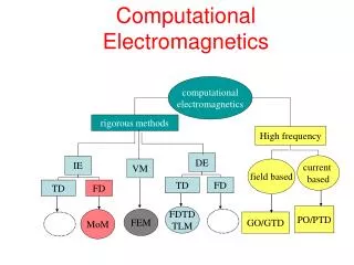
5. I. Introduction Numerical methods • Finite difference time domain approach (FDTD) • Spectral domain approach (SDA) • Finite element method (FEM) • Integral equation (IE) • Mode matching technique Widely used technique Method of Moment (MoM)

6. Disadvantages 1) Slow convergence of Green’s functions 2) A large number of basis functions Used solutions Using the 2D discrete fast Fourier Transform (FFT) 1) 2D-FFT + Using the first few resonant modes’ current distributions 1,2) Nonuniform meshs for mixed potential integral equation (MPIE)

7. New solution SDA + 2D-NUFFT + Nonuniform meshs NUFFT : 1D  2D The core idea of the 1D-NUFFT: The q+1 nonzero coefficients.

8. accuracy The nonsquare 2D-NUFFT NUFFT : 1D  2D The square 2D-NUFFT Some of these 2D coefficients approach to zero rapidly. The (q+1)2 nonzero coefficients. remove directly coefficients accuracy least square error

9. 2D-FFT II. 2D-NUFFT Algorithm Our aim (3.1) The key step (3.2) 2D-NUFFT (3.3)

10. Fr & Pr : closed forms Regular Fourier Matrix For a given (xt,ys), for m = -M/2,…,M/2-1 and n = -N/2,…, N/2-1 A: (MN)(q2/2+3q+1) b : (MN)1 Ar(xt,ys) = b(xt,ys)   r(xt,ys) = [A*A]-1[A*b(xt,ys)] = Fr-1Pr (3.5) where Fr is the regular Fourier matrix with size (q2/2+3q+1)2

11.  The [g(q+1)+(p+1)]throw ofFfequalsVpVg. Solution Extract Fr and Pr from Ff and Pf where Ff is the regular Fourier matrix with size (q+1)2 1)Define a vector product  as [a1, a2, …, am]  [b1, b2, …, bn] = [a1b1, a2b1, …, amb1, …, a1bn, a2bn, …, ambn] (3.6) Let Vp and Vg be the (p+1)th and (g+1)th row of the regular Foruier matrix for 1D problem p and g = 0, 1, …,q.

12. Let= ei2/cMand= ei2/cN, (3.7) (3.8)

13. 2)Choosemn = cos(m/cM)cos(n/cN).  The [g(q+1) +(p+1)]thelement ofPf (3.9) where {x} = x- [x].

14. Fr(i, j) = Ff((i), (j)) Pr(i) = Pf((i)) 3) FillFrand PrfromFfandPf For square grid points:  = [1, 2, …, (q+1)2] For octagonal grid points:  = [q/2, q/2+1, q/2+2, 3q/2, …, q2+3q/2, q2+3q/2+1, q2+3q/2+2]

15. Index  = [4, 5, 6, 12, 13, 14, 15, 16, …, 76, 77, 78] The relation between Fr and Ff, and Pr and Pf Example: Let q = 8 Index  = [1, 2, 3, …, 79, 80, 81]

16. 2D-NUFFT 1~3) Ff, PfFr, Pr  rr = Fr-1 Pr (3.5) 4) 2D-FFT: (3.4) If M = N = 210 and c = 2, then a 2D-FFT with size cMcN uses 3.02 seconds (CPU:1.6GHz). 5) (3.3)

17. is the spectral domain Green’s function where III. Approach The Green’s functions substrate thicknesst box dimensionabc kxm = mp/a, kyn = np/b (3.10)

18. Spectral domain Green’s functions

19. Solution procedure Asymmetric rooftop functions and the nonuniform meshs J(x, y) = axJx(x, y) + byJy(x, y) (3.11) source load terminal load terminal

20. Asymmetric rooftop function Jx = Jxx(x, x)Jxy(y, y) (3.12) (3.14a) (3.14b)

21. Galerkin’s procedure Final MoM matrix (3.15) Trigonometric identities (3.16)

22. Procedure for evaluating the MoM matrix

23. III. Numerical Results Hairpin resonator er= 10.2, L1 = 0.7, L2 = 1.01, L3 = 2.74, L4 = 8, L5 = 6, w1 = 1, w2 = 1.19, g1 = 0.2 and g2 = 0.8. All dimensions are in mm.

24. Table 3.1 Comparison of CPU Time and L2 error of One Call of the 2D-NUFFT in Analysis of a Hairpin Resonator Comparison of Analyses of The Hairpin Resonator with Uniform and Nonuniform Grids Table 3.2.1

25. The measured and calculated S parameters of the hairpin resonator.

26. Normalized magnitudes of the current distribution on the hairpin resonator at 2.473 GHz. (a) |Jx(x,y)| (b) |Jy(x,y)|

27. Normalized magnitudes of the current distribution on the hairpin resonator at 2.397 GHz. (c) |Jx(x,y)| (d) |Jy(x,y)|

28. Interdigital capacitor er= 10.2, L1 = 8, L2 = 1.6, L3 = 0.8, L4 = 1.2, L5 = 7.9, d = 0.4, e = 0.4, g = 0.2 and s = 0.2. The thickness of substrate is 1.27. All dimensions are in mm. Comparison of Analyses of The Ingerdigital capacitor with Uniform and Nonuniform Grids Table 3.2.2

29. The measured and calculated S parameters of the interdigital capacitor.

30. Normalized magnitudes of the current distribution on the interdigital capacitor at 5 GHz. (a) |Jx(x,y)| (b) |Jy(x,y)|

31. Wideband filter L1 = 8, L2 = 0.56, L3 = 0.576, L4 = 0.69, L5 = 0.3605, L6 = 0.125, L7 = 0.125, L8 = 0.125, L9 = 5.19, L10 = 4.88, L11 = 0.38, L12 = 2.06, L13 = 1.9, L14 = 7.75, L15 = 11.3, t = 0.635, er = 10.8. All dimensions are in mm. Comparison of Analyses of The Wideband filter with Uniform and Nonuniform Grids Table 3.2.3

32. The measured and calculated S parameters of the wideband filter.

33. Normalized magnitudes of the current distribution at 6 GHz (a) |Jx(x,y)| (b) |Jy(x,y)|

34. VI. Conclusion • A 2D-NUFFT algorithm with octagonalinterpolated • coefficients are used to enhance the Computation. • The octagonal2D-NUFFT uses less CPU time than • the square 2D-NUFFT. • The L2 error of the octagonal2D-NUFFT is the same • as that of square 2D-NUFFT. • The scattering parameters of the hairpin resonator, • an interdigital capacitor and a wideband filter are • calculated and validated by measurements.

35. THE END Thank You for your Participation !