粉體粒徑分析 Particle size analysis
Che5700 陶瓷粉末處理. 粉體粒徑分析 Particle size analysis. powder, particle (primary, secondary), colloid, agglomerate (soft, hard), aggregate, granule, crystallite: slightly different meaning Either single particle or a particle system is measured

粉體粒徑分析 Particle size analysis
E N D
Presentation Transcript
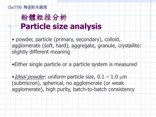
Che5700 陶瓷粉末處理 粉體粒徑分析Particle size analysis • powder, particle (primary, secondary), colloid, agglomerate (soft, hard), aggregate, granule, crystallite: slightly different meaning • Either single particle or a particle system is measured • Ideal powder: uniform particle size, 0.1 – 1.0 m (submicron), spherical, no agglomerate (or weak agglomerate), high purity, batch-to-batch consistency
Many possible particle shapes: rod, fiber, flake, tube (CNT), flower-like, etc. • If not spherical: need more than one parameter to describe the particle
Che5700 陶瓷粉末處理 Sampling • Be representative!! Need knowledge from statistical theory • different particles (shape, size, density etc.) – different motion, should be considered during sampling. • Golden Rules of Sampling: (a) samples should be in motion; (b) The whole stream of powder should be taken for many short increments of time in preference to part of the stream being taken for the whole time. • Results highly dependent on sampling techniques!!
Grab sample; cone & quarter; Riffling (three experimental methods) From JS Reed, 2nd ed.
Che5700 陶瓷粉末處理 Sampling Accuracy • Maximum sampling error: E = 2i/P where i = standard deviation from this sampling; P = weight fraction of material greater than 44μm (40 ppm here) • t = (i2 + n2) ½ where n = standard deviation from measurement; i.e. sampling error + measurement error
error size From JS Reed
Two-Component Sampling Accuracy • If we count particles (instead of measuring weight), then sampling error • σi = [p (1-p)/Ns (1- Ns/Nb)] ½ where p = fraction of particles above a certain size Ns = number of particles counted Nb = number of particles in the bulk This equation can also be used in estimating error from public opinion polls;
Che5700 陶瓷粉末處理 Different definitions of particle size • Principal concept: equivalent diameter to a sphere; • Equivalent items: e.g. volume, surface area, sedimentation velocity, projected area, (many kinds). • dv volume diameter V = /6 dv3 need particle volume • ds surface diameter S = ds2 .need particle surface • dvs surface volume diameter dsv = dv3/ds2 ..measure specific surface area of particle (per unit volume or unit weight) • Stoke’s diameter dStksame sedimentation velocity as a sphere
Che5700 陶瓷粉末處理 Different definitions of particle size(2) • projected area A = /4 da2 • Sieve diameter: passing opening of a sieve (width of square opening) • Martin diameter: mean chord length of projected outline of particle • Feret’s diameter: mean value of distance between pairs of parallel tangents to the projected outline of particles • We often use software to help with analysis of projected images (from SEM, TEM)
Martin diameter: in reality, we can choose several different directions and average the data • Feret diameter: distance between parallel tangents • Statistical diameter
Coulter counter: Principle when each particle passing through the aperture, it will displace same volume of conducting liquid, resistance then rise the frequency and extent of rise particle size and distribution Problem: two particles passing at the same time, or continuous passing of two particles, particle too large or too heavy, electrolysis, aperture blockage etc.
Che5700 陶瓷粉末處理 Microscopic Method • The basis of all techniques, (seeing is believing)!! OM, SEM, TEM • Need standard particles for calibration (e.g. PS polystyrene monodispersed particle from emulsion polymerization) • in association with image analysis software: can handle large number of images, good statistical results • ASTM counting requirements: modal size class at least 25 particles, best 10 in each class, total no less than 100 particles; (another suggestion: 700 particles least)
Some Terminology • Rayleigh scattering: particle size much smaller than wavelength d<<λ Rθ = Iθ r2/Io = 8 π4α2/λ4 (1+ cos2θ), where α = polarisability = (no/2π)(dn/dc)(M/L); λ = wavelength of incident light; no = refractive index of solvent, dn/dc = change of RI due to concentration, M = molecular weight (measured value), L = Avogadro No. • particle size much greater than wavelength: opaque, only scattering, Fraunhofer diffraction • Mie scattering: interaction between particle and light (in general 10λ – λ/10)
Che5700 陶瓷粉末處理 Optical Methods (Optical counters) • Laser diffraction technique: each particle producing Fraunhofer diffraction effect when passing parallel laser light, intensity of diffracted light ~ (size)2; diffracted angle ~ size. Handles gas (aerosol) or liquid samples. • Sensing volume can be very small such that only one particle counted at a time.
取自粉粒體粒徑量測技術, 高立圖書1998 Forward scatter, side scatter, back scatter
Dynamic Light Scattering (DLS) • Also termed as Photon Correlation Spectroscopy (PCS); or Quasi-elastic Light Scattering QELS) • Electric-filed time correlation function obtained from the scattered light due to motion of particles was analyzed to evaluate the average decay rate: Γ= D q2 • D = diffusion coefficient of particles; • Stokes-Einstein equation: R = kBT/(6πηD) to get particle size (R) • q = (4πno/λo) sin(θ/2); no refractive index of solvent; λo = wavelength of light
PCS or DLS 基本上是量測粒子散射光的相對強度, detect difference between movement, use correlator to analyze data, complex mathematics
Uncertainty analysis by dynamic light scattering • source: 機械工業, No 288, 94-100, 2007 • factors of uncertainty: Boltzman constant, wavelength of laser, scattering angle, diffraction coefficient, viscosity of solution, etc. • Based on the experiences of the authors: (以PS standard particles) for 20nm, 100nm & 1000 nm; their uncertainty 3.2 nm, 6.2 nm & 48 nm respectively.
PVP PEG N-Lauroylsarcosine N-Lauroylsarcosine
Che5700 陶瓷粉末處理 Hydrodynamic Chromatography • Same as other chromatography technique, particles of different size will move at different speed through the column, to become separated and then detected; smaller particles affected more by wall, move at slower rate. disadvantage: low sample recovery (may be trapped), possible interaction between particle and packing material, excessive sample dispersion, relative low resolution etc.
Rf = (time of passage of marker)/ (time of passage of colloid) versus colloid size calibration
X-ray Line Broadening • From full width at half maximum of XRD peaks, estimate of crystallite size (an average number); need complex mathematical treatment to get size distribution. • Scherrer equation: d hkl = k /(o cos); k = constant (mostly taken as 0.9 or 1.0; o = width at half height; = x ray wavelength; = diffraction angle (notice 2 ) [in theory: βo2=βm2-βi2, βm = measured breadth, βi = instrument breadth] • Reasons for broadening: small grain size, strain (or disorder) inside, instrumental error - use single crystal (Si) for calibration
From JS Reed, 2nd ed. Good instrument and practice should obtain similar results, not easy for one method to dominate.
Che5700 陶瓷粉末處理 Shape Factor • Surface or volume shape factor: V = v d3; or S = s d2; = shape factor, dependent on size measurement; αv =π/6; αs = π • shpericity 球形度: = (surface area of a sphere having same volume)/(actual surface area of particle) = (d NV/d NS) 2 • similar definition: circularity = (perimeter of a circle having same area)/(actual perimeter) • aspect ratio (長軸比): for fibers, = (length/ diameter) or (longest to shortest dimension)
All particles are hydrous zinc oxide (from different precipitation conditions): Shapes are different
Different name for different shapes ψA/ψV index of angularity (shape factor based on area/shape factor based on volume) Acicular: slender and pointed, needle-like 常用於描述葉子的形狀
* 取自TA Ring, 1996; S/V = St/V . Dav ; 其中St/V = surface area/unit volume (specific surface area, similar to based on unit weight), an easy to measure item (BET data)
More Shape Factors • Dynamic shape factor = (d NV/ d st)2 ; same motion resistance as a shpere; d NV & d st = volume equivalent diameter based on number & Stoke’s diameter respectively; • = -½ ( = sphericity) • Simple way to quantify shape and can be related to other properties or processing variables
Che5700 陶瓷粉末處理 Fractal Shapes • texture like a broccoli or cauliflower, the particle is fractal; then use fractal shapes, C = circumference (週線) estimated with a ruler of size Cx ~ x 1-D , where D = fractal dimension of particle • In a particle microscopic picture: number of particles in a circle of radius r plot log-log figure (N vs r), slope fractal dimension • Fractal shapes traditionally produced by agglomeration from sol-gel, or flame, plasma synthesis of ceramic powders • particle property related to fractal dimension, e.g. ~ R D-3; A ~ (ro)-1 R D; (ro = radius, R agglomerate size)
Che5700 陶瓷粉末處理 Size Distributions • expressions: (a) as a figure – (i) cumulative (oversize or undersize); or (ii) frequency – based on number, weight or volume, etc. (b) proper mathematical equations • CNPF: cumulative distribution based on number, percentage finer; CNPL (L = larger than this size) • CMPF: (M for weight) (based on weight)
Size interval: linear or geometric (幾何級數or log scale), e.g. 2 ½
Che5700 陶瓷粉末處理 Mathematical Equations • Two most popular equations: • Normal distribution: f(x) = 1/(2) exp[-(x – x)2/22] (two adjustable parameters): x & (average and standard deviation) ∫f(x) dx [from -∞ to ∞] = 1; σ=x(84.13) – x(50) = x(50) – x(15.87) • Log-normal distribution: f(z) = 1/(z2) exp[-(z – z)2/ 2z2] ; z = ln d (similar two parameters) or as f(d) = 1/(lng 2) exp[- (ln(d/dg))2/ 2 (lng)2] dgg = geometric mean size & standard deviation; σg = d 84.13/d 50 = d 50/d 15.87
Che5700 陶瓷粉末處理 More Equations • Rosin – Rammler distribution: f(x) = n b x (n-1) exp( - b xn) ; n & b adjustable parameters, related to particle characteristics, after integration, we get: F(x) cumulative distribution = exp( - b xn) …a simple equation • Gaudin – Schulmann model: w(d) = a n d (n-1) ; w(d) based on weight • Most equations have two parameters, similar results in fitting the true distribution, important question = what is the meaning of the parameters, any physical meaning.
From TA Ring, 1996; bimodal distribution Obtained from mixing of two particles with different size distributions, or one type particle from two different formation mechanisms
Che5700 陶瓷粉末處理 Mean diameters • Can use “mean”, “modal” (most populous) or median (in the middle or50%) • Mean (or average): several different ways (equations) to calculate it
fN(a): number distribution of size a; we can also have number mean diameter
Number frequency distribution (n) will be very much different from mass frequency distribution (nd3)
* From TA Ring, 1996; e.g. if expect 1% error, for a size interval having 20wt%, we need to count about 400 particles; total error = sampling error + sizing (analysis) error
Determine Error of Size Distribution (previous table) • 16-22 μm size interval: Wj = 13%, Nj = 110; Ej = error = Wj/(√Nj)= 1.2% • largest error: 60-84 size interval, only 1 particle counted, Wj = 6.5%, (from figure) Ej = 5% (?) • total error = ET = ΣEj Wj ~ 2% for this case
Che5700 陶瓷粉末處理 Characteristics of Agglomerates • Binding between particles: electrostatic, magnetic, van der Waals, capillary adhesion, hydrogen bonding, solid bridge (from atom diffusion) due to sintering, chemical reaction, dissolution-evaporation etc. • strength: may be estimated by methods such as compaction, ultrasonic vibration (indirect); size distribution before and after treatment get an estimation, in theory can be obtained from: primary particle size, coordination number, agglomerate porosity etc.