Chapter 5 Flow Analysis Using Control Volume (Finite Control Volume Analysis )
Chapter 5 Flow Analysis Using Control Volume (Finite Control Volume Analysis ). Many practical problems in fluid mechanics require analysis of the behavior of the contents of a finite region in space (a control volume). for example,

Chapter 5 Flow Analysis Using Control Volume (Finite Control Volume Analysis )
E N D
Presentation Transcript
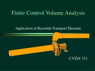
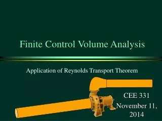
Chapter 5 Flow Analysis Using Control Volume (Finite Control Volume Analysis)
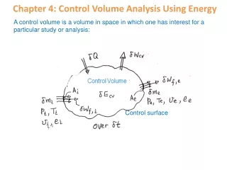
Many practical problems in fluid mechanics require analysis of the behavior of the contents of a finite region in space (a control volume). for example, to determine the amount of time to allow for complete filling of a large storage tank. to estimate of how much power it would take to move water from one location to another at a higher elevation and several miles away may be sought.
The bases of this analysis method are some fundamental principle of physics , namely , Conservation of mass Newton’s second law of motion , and the first and second laws of thermodynamics. • The finite control volume formulas are easy to interpret physically and are not difficult to use.
§ 5.1 Conservation of Mass-The continuity Equation • §5.1.1 Derivation of the continuity Equation
time rate of change of the mass of the coincident system time rate of change of the mass of the contents of the coincident c.v. net rate of flow of mass through the control surface = +
time rate of change of the mass of the coincident system time rate of change of the mass of the contents of the coincident c.v. net rate of flow of mass through the control surface = + t = t-δt t = t t = t+δt
§ 5.1.3 Moving, Non-deforming Control Volume • Example of moving, non-deforming control volume ---Control volumes containing a gas turbine engine on an aircraft in flight, and gasoline tank of an automobile passing.
§ 5.1.4. Deforming Control Volume • A deforming Control volume ~Changing volume size & control surface movement.
§ 5.2 Newton’s Second Law--The linear momentum and moment-of-momentum equations. • Newton’s second law of motion for a system is =>Any reference or coordinate system for which this statement is true is called inertial. A fixed coordinate system is inertial. A coordinate system that moves in a straight line with constant velocity and is thus without acceleration is also inertial.
When a control volume is coincident with a system at an instant of time, the forces acting on the system and the forces acting on the contents of the coincident control volume are instantaneously identical, that is,
Furthermore, for a system and the contents of a coincident control volume that is fixed and non-deforming, the Reynolds transport theorem allows us to conclude that
For a control volume that is fixed (inertial) and non-deforming, Eq.(5.19),(5.20), and (5.21) suggest that an appropriate mathematical statement of Newton’s Second law of motion is • Eq(5.22) is the linear momentum equation for a fixed, non-deforming control volume. Body force -- gravity only Surface force -- exerted on the contents of the control volume by material just outside the control volume in contact with material just inside the control volume
Several important notes: (1) 1-D flow problem when the flow is uniformly distributed over a section of the C.S. (2) Linear momentum is directional –three orthogonal coordinate directions. (3) Flux term is linear momentum─ • for Steady flow (In the textbook ,it is aussmed: Steady flow for the momentam problem) (5) If control surface ⊥ direction of flow Surface force exerted at these locations by fluid outside the C.V. on fluid inside will be due to pressure.
(6) Uniform pressure on control volume (7) Positive external force if the force is in the assigned positive coordinate direction. Negative otherwise. (8) Only external forces acting on the contents of the control volume are considered in the linear momentum equation.(Eq.5.22)
For a system and an inertial , moving , non-deforming control volume that are both coincident at an instant of time , the Reynolds transport theorem leads to This is the linear momentum equation for an inertial, moving, non-deforming control volume that involves steady flow.
§ 5.3 First Law of Thermodynamics-The Energy equation §5.3.1 Derivation of the Energy Equation • The first law of thermodynamics for a system is, in word ----(5.56)
Eq.(5.55) is valid for inertial and non-inertial reference system For the control volume that is coincident with the system at an instant of time