Download
1 / 24
240 likes | 401 Vues
Chapter 10--Costs of the Firm. Chapter Outline Costs In The Short Run Allocating Production Between Two Processes The Relationship Among MP, AP, MC, And AVC Costs In The Long Run Long-run Costs And The Structure Of Industry The Relationship Between Long-run And Short-run Cost Curves. 10- 1.

E N D
Chapter 10--Costs of the Firm Chapter Outline • Costs In The Short Run • Allocating Production Between Two Processes • The Relationship Among MP, AP, MC, And AVC • Costs In The Long Run • Long-run Costs And The Structure Of Industry • The Relationship Between Long-run And Short-run Cost Curves 10-1
Figure 10.1: Output as a Functionof One Variable Input [Chapter 9] DRTS 10-2 IRTS CRTS
Figure 10.2: The Total, Variable,and Fixed Cost Curves • Note: • similar curvature of TC and VC: VC=0 if Q=0 • Before Q=43 -> IRTS, thus VC increases at a decreasing rate • After Q=43, DRTS, VC increases at an increasing rate TCQ = FC + VCQ = rK0 + wL where TCQ, VCQ indicate that costs depend on output unlike FC which is independent of Q. Fixed cost (FC):cost that does not vary with the level of output in the short run (the cost of all fixed factors of production). Variable cost (VC):cost that varies with the level of output in the short run (the cost of all variable factors of production). Total cost (TC):all costs of production= the sum of variable cost and fixed cost. 10-3
Figure 10.3: The Production Function Q = 3KL, with K = 4 (CRTS) Slope =∆Q/∆L =12 10-4
Average Costs In The Short Run • Average fixed cost (AFC):fixed cost divided by the quantity of output, AFCQ = rKo/Q =FC/Q • Average variable cost (AVC):variable cost divided by the quantity of output, AVCQ = wL/Q=VCQ/Q • Average total cost (ATC):total cost divided by the quantity of output, ATC = AVC + AFC= (wL+rKo)/Q = TCQ/Q • Marginal cost (MC):change in total cost that results from a 1-unit change in output, MC = ∆TCQ/Q = ∆VCQ/Q since ∆FC/Q = 0 Graphing The Short-run Average and Marginal Cost Curves • Geometrically, average variable cost at any level of output Q may be interpreted as the slope of a ray to the variable cost curve at Q . 10-5
Figure 10.5: The Marginal, Average Total, Average Variable, and Average Fixed Cost Curves The MC intersects both the ATC and the AVC at their minimums 10-6
Marginal Costs • Is the same as the cost of expanding output (or the savings from contracting). • By far the most important of the seven cost curves. Reason: a typical firm makes a marginal decision whether to expand or contract production. This involves cost-benefit analysis (CBA). • Geometrically, at any level of output may be interpreted as the slope of the total cost curve at that level of output. • And since the total cost and variable cost curves are parallel, it is also equal to the slope of the variable cost curve. Marginal and Average Costs -When MC is less than average cost (either ATC or AVC), the average cost curve must be decreasing with output; and when MC is greater than average cost, average cost must be increasing with output. 10-8
Figure 10.7: Cost Curves for a Specific Production Process : Q= 3KL ,K=4 Given that Q= 3KL ,K=4, so Q =3*4L = 12L and L = Q/12, w=$24, r=$2, thus TCQ = wL +rK0 =2*4 + 24(Q/12) = 8 + 2Q Thus, TCQ= 8 + 2Q so that ATCQ = (8+2Q)/Q = 8/Q + 2 FC = $8 so that AFCQ = 8/Q VC =2Q so that AVC = 2Q/Q =2 and MC =∆TCQ/∆Q = 2 – slope of the TCQ ATC = TCQ=/Q = AVC +AFC = 2 + 8/Q 10-9
Figure 10.9: The Relationship Between MP, AP, MC, and AVC • Chap.9: MPL cuts the APL at the maximum value of the APL. • Chap. 10: MCQ cuts the AVC at the minimum value of the AVC. • These relationships serve a vital link for day-to-day management of a profit-maximizing firm: productivity (Chap. 9) is inversely linked to cost-control – a crucial understanding in all Accounting courses! • MCQ = ∆VCQ/∆Q and if Q= f(L), then ∆VCQ = ∆wL so that ∆VCQ/∆Q = ∆wL/∆Q. Given a fixed wage (w), then w∆L/∆Q = w/MPL = MCQ • The same reasoning applies to AVC = w/APL 10-10
Figure 10.10: The Isocost Line Given: w=$4, r =$2 and C= $100 Thus, wL + rK =C K= C/r - (w/r)*L –Isocost for the firm ≈ Budget Constraint for the Consumer 4L +2K= 100 w∆L + r∆K = ∆C =0 -w∆L= r∆K -w/r = ∆K/∆L =-4/2=-2 • Costs In The Long Run • Isocost line:a set of input bundles each of which costs the same amount. • To find the minimum cost point we begin with a specific isoquant then superimpose a map of isocost lines, each corresponding to a different cost level. • --The least-cost input bundle corresponds to the point of tangency between an isocost line and the specified isoquant. 10-11
Figure 10.11: The Maximum Outputfor a Given Expenditure 1. At B, MPL/MPK < PL/PK. In order to fix this, less labor and more capital is advised until the MPL/MPK = PL/PK at A. 2. At C, MPL/MPK >PL/PK. In order to fix this, more labor and less capital is advised until the MPL/MPK = PL/PK at A. 3. AtA, MPL/MPK = PL/PK. Thus, the firm is optimizing its employment of K at K* and L at L* to minimize its costs in producing Q0. C Firm should set MRTSL,K = -MPL/MPK = -w/r A B 10-12
Figure 10.12: The Minimum Costfor a Given Level of Output Firm should set MRTSL,K = -MPL/MPK = -w/r OR MPL/w = MPK/r 10-13
Figure 10.13: Different Ways of Producing 1 Ton of Gravel (Nepal) versus the US Gravel is made by hand in Nepal (isocost line), but by machine in the U.S.(isocost line) because the relative prices of labor and capital differ so dramatically in the two countries. That is, 10-14
Figure 10.15: The Long-Run Expansion Path Recall the (1) Price Expansion Path (PEP) and (2) Income Consumption (ICP) in case of the Consumer • The Relationship Between Optimal Input Choice And Long-run Costs • Output expansion path (OEP)- the locus of tangencies (minimum cost input combinations) traced out by an isocost line of given slope as it shifts outward into the isoquant map for a production process. 10-15
Figure 10.16: The Long-Run Total, Average, and Marginal Cost Curves • The Long-run MC =LMCQ = ∆LTCQ/∆Q • The long-run average cost, LACQ = LTCQ/Q • There are no fixed costs (FC) in the LR! • Plot (Q1, TCQ1), (Q2, TCQ2) and so forth from Figure 10.15 onto top Panel of Figure 10.16. • Since in the LR, there are no FCs this means that all costs are variable. • The long-run total cost (LTC) always passes through the origin since the firm can always liquidate all its inputs. 10-16
Figure 10.17: The LTC, LMC and LAC Curves for a PF exhibiting Constant Returns to Scale (CRTS) Constant returns to scale - long-run total costs are thus exactly proportional to output. 10-17
Figure 10.18: The LTC, LAC and LMC Curves for a Production Process with Decreasing Returns to Scale Decreasing returns to scale - a given proportional increase in output requires a greater proportional increase in all inputs and hence a greater proportional increase in costs. 10-18
Figure 10.19: The LTC, LAC and LMC Curves for a Production Process with Increasing Returns to Scale Increasing returns to scale - long-run total cost rises less than in proportion to increases in output Next: Examine the importance of long-run costs for the structure of an industry. 10-19
Figure 10.20: LAC Curves Characteristic of Highly Concentrated Industrial Structures Ever declining LAC is a cost advantage that allows an existing firm defensive barriers against possible competitors (barriers to entry) Industry dominated by a few firms if Q0 forms a substantial share for an industry. • Long-run Costs And The Structure Of Industry • Natural monopoly:an industry whose market output is produced at the lowest cost when production is concentrated in the hands of a single firm[Panel A]. • Minimum efficient scale: the level of production required for LAC to reach its minimum level, Q0 [Panel B]. 10-20
Figure 10.21: LAC Curves Characteristic of Unconcentrated Industry Structures • Survival in an industry requires a low-cost structure (U-shaped LAC) and if Q0 is small share for the industry, then many firms are in the industry (Panel A). • Similarly, if the LAC is flat (Panel B) or rising (Panel C), it is possible to have many firms, each producing a small portion of the industry output. • Industry – collection of firms that produce identically or similar products. 10-21
Figure 10.22: The Family of Cost Curves Associated with a U-Shaped LAC • The LAC is the “envelope” of all ATC curves • LMC = SMC at the value of output (Q2 in this case) where ATC is tangent to the LAC. • At the minimum point of the LAC, LMC = SMC = ATC = LAC • For Plant sizes 1 (ATC1) and 2 (ATC2), the SMC1 and SMC3 do not hit LAC or ATC at its minimum. • Only and only with Plant Size 2 (ATC2) does the LMC hit the ATC and LAC from below at its minimum. Plant Size 2 minimizes both SR and LR costs. 10-22
Figure A10.1: The Short-run and Long-Run Expansion Paths • OE is the LR expansion path • With K fixed at K = K2*, the SR expansion path is a horizontal line through point (0, K2*). • Given that K2* is the optimal K for producing Q = 2, the LR and SR expansion paths intersect at point T. • The SR TCQ of producing a given level of output is the cost given by the relevant isocost line. For example, for Q3, the SR TCQ is given by STC3 10-23
Figure A10.2: The LTC and STC Curves Associated with the Isoquant Map in Figure A.10.1 • As Q approaches Q=2 (the level of output for which the fixed factor is at optimal level), STCQ approaches LTCQ. • The STCQ and LTCQ curves are tangent at Q=2 • Beyond Q=2, STCQ increases faster than LTCQ due to diminishing returns that partly governs the behavior of STCQ in the SR. 10-24