Download
1 / 10
140 likes | 451 Vues
The Two-body Equation of Motion. Newton’s Laws gives us:. The solution is an orbit described by a conic section (circle, ellipse, parabola, or hyperbola) that is fixed in space The satellite will trade kinetic energy for potential energy (speed for altitude) as it moves around in orbit

E N D
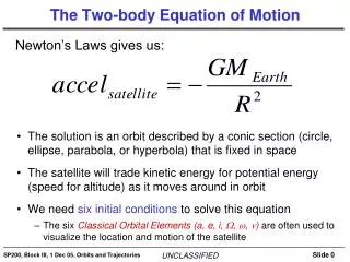
The Two-body Equation of Motion Newton’s Laws gives us: • The solution is an orbit described by a conic section (circle, ellipse, parabola, or hyperbola) that is fixed in space • The satellite will trade kinetic energy for potential energy (speed for altitude) as it moves around in orbit • We need six initial conditions to solve this equation • The six Classical Orbital Elements (a, e, i, W, w, n) are often used to visualize the location and motion of the satellite
Classical Orbital Elements Orbit Size: Semi-major Axis a Orbit Shape: Eccentricity e Orbit Tilt: Inclination i Orbit Twist: Right Ascension of Ω the Ascending Node Orbit Rotation: Argument of Perigee ω Satellite Location: True Anomaly
Size: Semi-Major Axis (a) US: Fig. 5-2 • How big is an orbit? We measure the length of the longest side of the ellipse and, by convention, divide it in half • Orbit size depends on how fast we “throw” our satellite into orbit • The faster we throw it, the more energy its orbit has and the bigger its orbit is
Shape: Eccentricity (e) e = .8 e = .5 e = .7 US, Fig. 5.3 e = 0 (circular) Circle e = 0.0 Ellipse e = 0.0 to 1.0 Parabola e = 1.0 Hyperbola e > 1.0
Tilt: Inclination (i) Inclination K h i Angular momentum vector Equatorial Plane
Tilt: Inclination (i) US: Table 5-2
Twist: Right Ascension of the Ascending Node () Vernal Equinox Direction (Originally pointed to the constellation Aries, the Ram) Equatorial Plane Ascending Node Right Ascension of the Ascending Node (Also called the Longitude of the Ascending Node) We measure how an orbit is twisted by locating its ascending node relative to the vernal equinox direction (in the equatorial plane)
Rotation: Argument of Perigee () Argument of Perigee Equatorial Plane Ascending Node Perigee (Point Closest to the Earth) We locate perigee relative to the ascending node (in the orbit plane)
Satellite Location: True Anomaly () Equatorial Plane True Anomaly Perigee (Point Closest to the Earth) Finally, we locate the satellite relative to perigee, (in the orbit plane)
Classical Orbital Elements w 2a K i e = .8 h Vernal Equinox Direction Ascending Node Perigee