Modeling
Modeling. A model is an abstraction of reality No model can include all the complexity of the real world. Hopefully a model includes enough complexity from the real world to adequately represent the system.

Modeling
E N D
Presentation Transcript
Modeling • A model is an abstraction of reality • No model can include all the complexity of the real world. Hopefully a model includes enough complexity from the real world to adequately represent the system. • As model complexity increases so does the resources needed to use the model ($$) and the chances for uncertainty (more variables that can be wrong). • All GIS is a modeling exercise.
Types of Models • Types of Models • Physical: tangible representation • Models of dams, airplanes, etc. • Theological: logical or mathematical representation • GIS models are theological • Level of Theory • Empirical: based solely on data (e.g. regression). • Biophysical (social-economic): based solely on basic principles. Also called theologically-based. • Conceptual (or Hybrid) – usually has theological framework with empirical derived parameters. The empirical parameter provides for natural variability. • Most cartographic models are conceptual
USCAE San Francisco Bay Model http://www.spn.usace.army.mil/bmvc/
Models based on logic • Logic is used in the conceptualization and formulation of the model. • Inductive logic: build models based on individual data or instances. This is done by employing empirical tests. Requires data! • Deductive logic: based on known premise of the important factors and interactions. Moves from general knowledge to specific outcomes through conceptualization, formulation, flow-charting, and implementation of the model.
Types of Models • Methodology • Stochastic: based on statistical probabilities • Potential for many outcomes with the same input. • Deterministic: based on known functional linkages and interactions • Only one potential outcome with a given input • They can be linked. • A deterministic hydrologic model can be linked to a stochastic weather generator to provide stochastic results (i.e. a potential range of flows from a give landscape configuration)
Y = a + b * X Y Y = a + b *X + έ X
Time • Static modeling utilizes a single realization or slice of time of a physical process or description of the landscape given the existing conditions (for example, a suitability model). The static approach can be either deterministic or stochastic. • Dynamic modeling is an approach in which pieces of a model, or the entire model, are rerun with the output of the model becomes the input for the next iteration of the model. Usually, in dynamic GIS models, time and space are explicitly modeled. The dynamic approach can be either deterministic or stochastic.
Management Applications of GIS • Graphics and Visualization • Spatial Database Management System • Spatial Analysis (including statistics) • Modeling • -Cartographic Modeling (within GIS)*-Interface and DBMS for standalone models
Map Products for Decision-Making Raw Data Analysis Modeling - “Synthesis” Interpretation Information
1. Current Conditions Representing current conditions for important thematic variables maybe the most common application. All planning efforts require a description of the “starting point”, what resources are available and what problems exist. Raw data can be represented different ways (normalization, indices) to help in interpretation. 2. Change Analysis Comparison between past vs. current conditions. Isolating areas of concern due to changes. Example: Delineate areas that have developed over the past decade to identify areas with potential water quality problems.
Land cover change on the Upper San Pedro - NALC classification data 1973 1986 1992 1997
Grassland Fragmentation Index 1997 1973 Courtesy Bill Kepner, US-EPA
Human Use Index 1973 1997 Area near Sierra Vista, AZ Fast-growing city Courtesy Bill Kepner, US-EPA
3. Future Scenario Simulation Develop models to forecast future conditions that may be used to predict potential impacts. Examples: Projection of future growth rates to assess if the current infrastructure is adequate. One way this can be accomplished by taking the current zoning and then evaluate that would happen if the land was developed (full build-out) at its potential density (# houses/area) or economic use (residential vs. commercial). What would happen if zoning were changed (e.g. higher densities)? How would this affect flooding and floodplains? Predict potential deforestation with potential new roads.
Urban Growth Modeling The SLEUTH Model SLEUTH belongs to the cellular automata class of models, so the study area is represented as a regular grid of cells and each cell has only two states: urbanized or non-urbanized. The current version of SLEUTH is not capable of modeling density of development within a pixel. Whether or not a cell will become urbanized is determined by four growth rules, each of which attempts to simulate a particular aspect of the development process.
Urban Growth Modeling SLEUTH simulates four types of growth, which areapplied sequentially during each growth cycle : • Spontaneous new growth, which simulates the random urbanization of land, • New spreading centers, which simulates the development of new urban areas, • Edge growth, which stems from existing urban centers, • Road influenced growth, which simulates the influence of the transportation network on development patterns.
Campbell et al. http://gis.esri.com/library/userconf/proc01/professional/papers/pap324/p324.htm
4. Assessment of Hazards – delineating areas with high vs. low risk. Erosion Hazard Landslide Hazard Flooding Water Quality Impairment Potential for groundwater contamination (Drastic Mapping) Health risks due to pollution Hazards usually represent constraints to other land uses or activities. Used to delineate/define areas for Best Management Practices (BMPs).
Regional Ground Water Vulnerability – Detail (1500m x 1500m) Scale Potential Risk for Nitrates – Use of Logistic Regression
Watershed Classification: Selenium Example One common source of elevated selenium in the western United States is flood irrigation drainage from seleniferous soils. The fuzzy logic classification for selenium in each subwatershed of this Upper Gila Watershed example was created based on ADEQ water quality assessment data and the percentage of agricultural land in each subwatershed.
5. Assessment of Potential – delineating areas have a high or low promise of a potential outcome. Similar to hazard. Examples: Archeological sites – probability of occurrence. Deforestation – probability of occurrence Potential crop yield (kg/ha) under different condition
Deforestation Probability Surface • Cell by Cell Logistic Regression for Each Analysis Year (1986 to 1999) using 5 % Stratified Random Samples (> 1,100,000 cells): • Dependent Variable: Deforested (1) / Forested (0) • Independent Variables: LN distance to Roads, LN Distance to Settlements, Well (1) / Poorly (0) Draining Soils
1986 - Deforestation Probability Surface Results 1986 Observed Deforestation
1995 - Deforestation Probability Surface Results 1995 Observed Deforestation
6. Suitability Analysis – delineating areas based on their appropriateness to support for an activity. This is also referred to as Site or Location analysis. Examples: Wildlife habitat suitability (usually species specific) Locating the sites for a business Locating the path for a road/trail/power line Suitability for use as irrigated cropland Ability to support riparian restoration activities
http://www.innovativegis.com/basis/MapAnalysis/MA_Intro/MA_Intro.htmhttp://www.innovativegis.com/basis/MapAnalysis/MA_Intro/MA_Intro.htm
7. Capability Analysis – delineating areas based on their suitability to support difference sets of activities. Examples: Land Use Zoning - usually presented as a hierarchy of activities with increasing constraints If an area is zoned to medium density residential (<= 2 houses/ac) it can be used for low density residential (<= 1 house /ac) or rural residential (<= 0.25 house / ac). However, if something is zoned “open space” it cannot be developed. But note that: To some people a zoning map represents the “potential” since it is assumed you would want to develop the land for the maximum profit. If you are dealing with only one activity suitability and capability are the same.
Methods 1. Gestalt (user defined) 2. Logic/Rule Approach (Qualitative) Exclusion – remove areas based on policy/conditions 3. Model – based on a theoretical or empirical model of the system (e.g. Universal Soil Loss Equation) 4. Statistical Approaches - Bayesian statistics - Classification methods (clustering or PCI) - Classification Regression Trees (CART) - Regression (e.g logistic – probability of occurrence)
5. Map Overlay Approaches – the combination of different factors to create an ordinal (rank) map. - Boolean - Ordinal Combination - Linear Combination (with weights) 6. Optimization Approaches - Shortest Path – Network Analysis - Multi-criteria - Fuzzy Logic - AHP - Neural Networks/ Genetic Algorithms