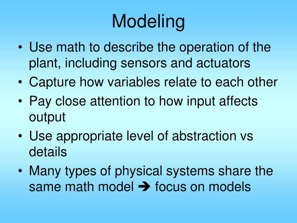
1. Modeling • Use math to describe the operation of the plant, including sensors and actuators • Capture how variables relate to each other • Pay close attention to how input affects output • Use appropriate level of abstraction vs details • Many types of physical systems share the same math model  focus on models

2. Modeling Guidlines • Focus on important variables • Use reasonable approximations • Write mathematical equations from physical laws, don’t invent your own • Eliminate intermediate variables • Obtain o.d.e. involving input/output variables  I/O model • Or obtain 1st order o.d.e.  state space • Get I/O transfer function

3. Common Physical Laws • Circuit: KCL: S(i into a node) = 0 KVL: S(v along a loop) = 0 RLC: v=Ri, v=Ldi/dt, i=Cdv/dt • Linear motion: Newton: ma = SF Hooke’s law: Fs = KDx damping: Fd = CDx_dot • Angular motion: Euler: Ja = St t = KDq t = CDq_dot

4. More Physical Laws

5. Electric Circuits Voltage-current, voltage-charge, and impedance relationships for capacitors, resistors, and inductors impedance admittance

6. RLC network KVL:

7. Or start in s-domain and solve for TF directly

8. Zf Iin=0  Zi Vin=0 Gain = inf Ideal Op amp:

9. Mesh analysis Mesh 2 Mesh 1

10. Write equations around the meshes Sum of impedance around mesh 1 Sum of applied voltages around the mesh Sum of impedance common to two meshes Sum of impedance around mesh 2

11. Determinant

13. Nodal analysis i3 i1 Kirchhoff current law at these two nodes i2 i4 i1 - i2 - i3=0 i3 - i4 =0

14. Kirchhoff current law conductance

15. Sum of injected current into each node Sum of admittance at each node Admittance between node i and node j