Download
1 / 52
540 likes | 601 Vues
Explore the fields of Computer Vision, Computer Graphics, and Image Processing, understanding how to extract scene information from 2D images and videos. Discover the mathematical concepts behind projection matrices, camera models, and projective transformations, transforming 2D images into 3D models. Dive into tasks in Geometric Vision such as tracking, visual control, 3D reconstruction, and structure from motion. Learn about reconstructing scenes, modeling scenes of various scales, and refining reconstructions using stereo techniques. Delve into the world of city modeling, architectural elements, and interactive systems in Computer Vision.

E N D
What is Computer Vision? Computer Vision Computer Vision Computer Graphics Image Processing • Three Related fields • Image Processing: Changes 2D images into other 2D images • Computer Graphics: Takes 3D models, renders 2D images • Computer vision: Extracts scene information from 2D images and video • e.g. Geometry, “Where” something is in 3D, • Objects “What” something is” • What information is in a 2D image? • What information do we need for 3D analysis? • CV hard. Only special cases can be solved. 90 horizon
The equation of projection Mathematically: Cartesian coordinates: • Intuitively: • Projectively: Projection matrix Camera matrix (internal params) Rotation, translation (ext. params)
The 2D projective plane X x X X Y y Y Y 0 Z Z l∞ Projective point X∞ Homogeneous coordinates s s 0 X 1 Inhomogeneous equivalent = Z Y • Perspective imaging models 2d projective space • Each 3D ray is a point in P2 : homogeneous coords. • Ideal points • P2 is R2 plus a “line at infinity” X∞ = l∞
Lines X Y Z X A 0 Y 0 B 0 1 C For any 2d projective property, a dual property holds when the role of points and lines are interchanged. Duality: l = X1 X2 l1 l2 X = • Projective line ~ a plane through the origin l = = X lTX = XTl = AX + BY + CZ = 0 X l∞ l = X∞ = “line at infinity” • Ideal line ~ the plane parallel to the image HZ The line joining two points The point joining two lines
Projective transformations • Homographies, collineations, projectivities • 3x3 nonsingular H maps P2 to P2 8 degrees of freedom determined by 4 corresponding points • Transforming Lines? subspaces preserved substitution dual transformation
Planar Projective Warping HZ A novel view rendered via four points with known structure
Geometric strata: 2d overview l ¥ C* C* ¥ ¥ 2 dof l ¥ 2 dof
Projective 3D space • Points Points and planes are dual in 3d projective space. • Planes • Lines: 5DOF, various parameterizations • Projective transformation: • 4x4 nonsingular matrix H • Point transformation • Plane transformation • Quadrics:Q Dual: Q* • 4x4 symmetric matrix Q • 9 DOF (defined by 9 points in general pose)
Geometric strata: 3d overview 3DOF 5DOF Faugeras ‘95
Tasks in Geometric Vision 1 y1 1 y3 1 y2 • Tracking: Often formulated in 2D, but tracks 3D objects/scene • Visual control: Explicit 2D geometric constraints implicitly fulfills a 3D motion alignment • 3D reconstruction: Computes an explicit 3D model from 2D images
Camera model: Relates 2D – 3D [Dürer] Projection matrix Camera matrix (internal params) Rotation, translation (ext. params)
2D-3D geometry - resection • Projection equation xi=PiX • Resection: • xi,X Pi Given image points and 3D points calculate camera projection matrix.
2D-3D geometry - intersection • Projection equation xi=PiX • Intersection: • xi,Pi X Given image points and camera projections in at least 2 views calculate the 3D points (structure)
2D-3D geometry - SFM • Projection equation xi=PiX • Structure from motion (SFM) • xi Pi,X • Given image points in at least 2 views calculate the 3D points (structure) and camera projection matrices (motion) • Estimate projective structure • Rectify the reconstruction to metric (autocalibration)
Reconstructing scenes ‘Small’ scenes (one, few buildings) • SFM + multi view stereo • man made scenes: prior on architectural elements • interactive systems City scenes (several streets, large area) • aerial images • ground plane, multi cameras SFM + stereo [+ GPS] depth map fusions
Large scale (city) modeling Modeling dynamic scenes time
Modeling (large scale) scenes [Adam Rachmielowski ]
SFM + stereo • Man-made environments : • straight edges • family of lines • vanishing points [Dellaert et al 3DPVT06 ] [Zisserman, Werner ECCV02 ]
SFM + stereo • dominant planes • plane sweep – homog between 3D pl. and camera pl. • one parameter search – voting for a plane [Zisserman, Werner ECCV02 ] [Bischof et al 3DPVT06 ]
SFM + stereo • refinement – architectural primitives [Zisserman, Werner ECCV02 … ]
SFM+stereo • Refinement – dense stereo www.arc3d.be [Pollefeys, Van Gool 98,00,01]
Façade – first system Based on SFM (points, lines, stereo) Some manual modeling View dependent texture [Debevec, Taylor et al. Siggraph 96]
Priors on architectural primitives prior θ – parameters for architectural priors type, shape, texture M – model D – data (images) I – reconstructed structures (planes, lines …) [Cipolla, Torr, … ICCV01] Occluded windows
Interactive systems Video, sparse 3D points, user input M – model primitives D- data I – reconstructed geometry Solved with graph cut [Torr et al. Eurogr.06, Siggraph07]
City modeling – aerial images Airborne pushbroom camera Semi-global stereo matching (based on mutual information) [Heiko Hirschmuller et al - DLR]
City modeling – ground plane Camera cluster Video: Cannot do frame-frame correspondences car + GPS 2D feature tracker Calibrated cameras – relative pose GPS – car position - 3D tracking SFM [Nister, Pollefeys et al 3DPVT06, ICCV07] [Cornelis, Van Gool CVPR06…] 3D points Dense stereo+fusion Texture 3D MODEL
City modeling - example [Cornelis, Van Gool CVPR06…] • 1. feature matching = tracking • 2. SFM – camera pose + sparse 3D points • 3. Façade reconstruction • – rectification of the stereo images • - vertical line correlation • 4. Topological map generation • - orthogonal proj. in the horiz. plane • - voting based carving • 5. Texture generation • - each line segment – column in texture space VIDEO
On-line scene modeling : Adam’s project • On-line modeling from video • Model not perfect but enough for scene visualization • Application predictive display • Tracking and Modeling • New image • Detect fast corners (similar to Harris) • SLAM (mono SLAM [Davison ICCV03]) • Estimate camera pose • Update visible structure • Partial bundle adjustment – update all points • Save image if keyframe (new view – for texture) • Visualization • New visual pose • Compute closet view • Triangulate • Project images from closest views onto surface SLAM Camera pose 3D structure Noise model Extended Kalman Filter
Modeling dynamic scenes [Neil Birkbeck]
Multi-camera systems time Several cameras mutually registered (precalibrated) Video sequence in each camera Moving object
Techniques • Naïve : reconstruct shape every frame • Integrate stereo and image motion cues • Extend stereo in temporal domain • Estimate scene flow in 3D from optic flow and stereo Representations : • Disparity/depth • Voxels / level sets • Deformable mesh – hard to keep time consistency Knowledge: • Camera positions • Scene correspondences (structured light)
Spacetime stereo [Zhang, Curless, Seitz: Spacetime stereo, CVPR 2003] Extends stereo in time domain: assumes intra-frame correspondences Static scene: disparity Dynamic scene:
Spacetime photometric stereo [Hernandez et al. ICCV 2007] One color camera projectors – 3 different positions Calibrated w.r. camera Each channel (R,G,B) – one colored light pose Photometric stereo
3. Scene flow [Vedula, Baker, Rander, Collins, Kanade: Three dimensional scene flow, ICCV 99] 3D Scene flow 2D Optic flow Scene flow on tangent plane Motion of x along a ray
Scene flow: results [Vedula, et al. ICCV 99]
Scene flow: video [Vedula, et al. ICCV 99]
4. Carving in 6D [Vedula, Baker, Seitz, Kanade: Shape and motion carving in 6D] Hexel: 6D photo-consistency:
6D slab sweeping Slab = thickened plane(thikness = upper bound on the flow magnitude) • compute visibility for x1 • determine search region • compute all hexel photo-consistency • carving hexels • update visibility (Problem: visibility below the top layer in the slab before carving)
7. Surfel sampling [ Carceroni, Kutulakos: Multi-view scene capture by surfel samplig, ICCV01] • Surfel: dynamic surface element • shape component : center, normal, curvature • motion component: • reflectance component: Phong parameters
Reconstruction algorithm ci – camera i ll- light l visibility Phong reflectance shadow
Modeling humans in motion Goal: 3D model of the human Instantaneous model that can be viewed from different poses (‘Matrix’) and inserted in anartificial scene (tele-conferences) Multiple calibrated cameras Human in motion • Our goal: 3D animated human model • capture model deformations and appearance change in motion • animated in a video game GRIMAGE platform- INRIA Grenoble
Articulated model Model based approach [Neil Birkbeck] • Geometric Model • Skeleton + skinned mesh (bone weights ) • 50+ DOF (CMU mocap data) • Tracking • visual hull – bone weights by diffusion • refine mesh/weights • Components • silhouette extraction • tracking the course model • learn deformations • learn appearance change