Download

1 / 18
190 likes | 445 Vues
Classification of Cancer Patients. Naomi Altman Nov. 06. The Prostate Cancer Data. I downloaded from GEO, 19 cel files, with 54000 genes. 6 benign tissue 6 primary tumors 7 metastatic tumors Normalized by RMA Used limma to compute F.p.value for differential expression.

E N D
Classification of Cancer Patients Naomi Altman Nov. 06
The Prostate Cancer Data I downloaded from GEO, 19 cel files, with 54000 genes. 6 benign tissue 6 primary tumors 7 metastatic tumors Normalized by RMA Used limma to compute F.p.value for differential expression. Wrote the data and q.values to cancerSig.txt
Some preliminaries We might want to start by clustering the samples or looking at the plots in the SVD directions (for the arrays). Since SVD and hclust both act on rows, we need to transpose the data matrix (and remember to eliminate the q-value column) groups=as.factor(colnames(sig.cancer)) plot(hclust(dist(t(sig.cancer[,1:19])))) svd.c=svd(t(sig.cancer[,1:19])) plot(svd.c$u[,1],svd.c$u[,2], col=as.numeric(groups))
Linear and Quadratic Discriminant Analysis The first 2 SVD directions do not entirely separate the samples, although we can see that we ought to be able to do this from the cluster analysis. But the cluster analysis does not give us a rule for classifying a new sample. So, lets try LDA and QDA, which can be found in the MASS library. library(MASS) lda.c=lda(t(sig.cancer[,1:19]),groups)
Linear and Quadratic Discriminant Analysis #Since R runs out of memory - cut down the number of genes - e.g. 100 gc() #you should always do this if you run out of memory lda.c=lda(t(sig.cancer[1:100,1:19]),groups)
Linear and Quadratic Discriminant Analysis #If the number of genes is greater than the number of samples, # the S matrix is singular, so the LDA function cannot be # computed! lda.c=lda(t(sig.cancer[1:12,1:19]),groups) plot(lda.c,col=as.numeric(groups)) # What is special about the first 12 genes? Nothing dim(sig.cancer) lda.c=lda(t(sig.cancer[sample(1:9299,12),1:19]),groups) plot(lda.c,col=as.numeric(groups))
Linear and Quadratic Discriminant Analysis #Any random set of genes in the file will separate the metastatic cancers from the others. #Some sets of genes will also separate the benign tumors from the primary cancers. #How can we choose a "good" set? and how many genes do we need in this set? Some ideas: # Use limma to compute the pairwise comparisons and take the 3 or 4 most significant genes from each comparison. # Look at lots of random sets and compute the misclassification rate for each (many are perfect). # Use a method like recursive partitioning which is stepwise.
Linear and Quadratic Discriminant Analysis #While we are here, lets try quadratic. qda.c=qda(t(sig.cancer[sample(1:9299,12),1:19]),groups)
Linear and Quadratic Discriminant Analysis #While we are here, lets try quadratic. qda.c=qda(t(sig.cancer[1:12,1:19]),groups) #QDA requires more data, because it needs to invert the within # group covariance matrix which has rank 1 less than sample size # We can try fewer predictors (genes) - 1 less than the minimum #sample size qda.c=qda(t(sig.cancer[1:5,1:19]),groups) predict(qca.c)
Recursive Partitioning library(rpart) rpart.c=rpart(groups~t(sig.cancer[,1:19])) plot(rpart.c) #rpart will not split groups that are already small. # 20 is considered small rpart.c=rpart(groups~t(sig.cancer[,1:19]), minsplit=5) plot(rpart.c) summary(rpart.c)
Recursive Partitioning #Again the choice of genes is pretty arbitrary rpart.c=rpart(groups~t(sig.cancer[sample(1:9299,100),1:19]), minsplit=5) plot(rpart.c) summary(rpart.c)
Prediction Analysis for Microarrays - PAM I downloaded pamr from the same site as SAM www-stat.stanford.edu/~tibs The package can be installed from the packages menu.
PAM #We need to format the data to pamr input pam.in=list(x=sig.cancer[,1:19], y=groups, genenames=rownames(sig.cancer), geneid=rownames(sig.cancer)) # We then "train" the data train.c=pamr.train(pam.in) #The centroids can be plotted at different cut-offs to see the "informative genes"
PAM pamr.plotcen(pamr.out, pam.in, threshold=10) pamr.plotcen(pamr.out, pam.in, threshold=4) #Cross-validation can be used to decide on a threshold cv.c<- pamr.cv(pamr.out, pam.in) pamr.plotcv(cv.c) #list the genes at the appropriate threshold pamr.listgenes(pamr.out,pam.in, threshold=8.0)
PAM #Unlike their example, we have lots of genes. Lets see if we can #reduce the number #The problem is the class that is easiest to predict - i.e. meta, so #lets just remove some of those genes from the data pam.gene=pamr.listgenes(pamr.out,pam.in, threshold=9.0) pam.keep=pam.gene[c(1:20,40:49,75),1] data.keep=which(pam.keep %in% pam.in$genenames) small.in=pam.in small.in$x=pam.in$x[data.keep,] small.in$y=pam.in$y[data.keep] small.in$genenames=pam.in$genenames[data.keep] small.in$geneid=pam.in$geneid[data.keep] • pamr.plotcv(small.cv) • pamr.plotcen(small.out,small.in,threshold=5.5)
small.out=pamr.train(small.in) pamr.cv(small.out,small.in) small.cv=pamr.cv(small.out, small.in) pamr.plotcv(small.cv) small.cv pamr.plotcen(small.out,small.in, threshold=2) # 2 errors with 25 genes # 1 error with 29 genes