Dick Bond
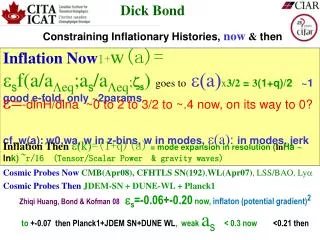
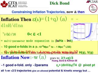
Dick Bond. Constraining Inflation Trajectories, now & then. Inflation Then k =(1+q)(a) = - dlnH / dlna ~r(k)/16 0< <1 = multi-parameter mode expansion in ( ln Ha ~ ln k ) ~ 10 good e-folds in a (k~10 -4 Mpc -1 to ~ 1 Mpc -1 LSS)

Dick Bond
E N D
Presentation Transcript
Dick Bond Constraining Inflation Trajectories, now&then Inflation Thenk=(1+q)(a) = -dlnH/dlna ~r(k)/16 0< <1 = multi-parameter mode expansion in (lnHa ~ lnk) ~ 10 good e-folds in a (k~10-4Mpc-1 to ~ 1 Mpc-1 LSS) ~ 10+ parameters? Bond, Contaldi, Huang, Kofman, Vaudrevange 08 H(f),V(f) ~0 to 2 to 3/2 to ~.4 now, on its way to 0? Inflation Now1+w(a) goes to2(1+q)/3 ~1 good e-fold. only ~2params es= (dlnV/dy)2/4 @ pivot pt all 1+w <2/3 trajectories give an allowed potential & kinetic energy but … Huang, Bond & Kofman 08
Standard Parameters of Cosmic Structure Formation r < 0.47 or < 0.2895% CL New Parameters of Cosmic Structure Formation
TheParameters of Cosmic Structure Formation Cosmic Numerology: aph/0801.1491 – our Acbar paper on the basic 7+; bchkv07 WMAP3modified+B03+CBIcombined+Acbar08+LSS (SDSS+2dF) + DASI (incl polarization and CMB weak lensing and tSZ) ns = .962 +- .014(+-.005 Planck1) .93 +- .03 @0.05/Mpcrun&tensor r=At / As < 0.47cmb95% CL (+-.03 P1) <.55 CMB+LSS eprior 5-pivot B-spline < .22 CMB+LSS lneprior 5-pivot B-spline dns /dln k=-.04 +- .02 (+-.005 P1) CMB+LSS run&tensorprior change?<#(1-ns) As = 22 +- 2 x 10⁻¹⁰ 1+w = 0.02 +/- 0.05 ‘phantom DE’ allowed?! +-.07 then Wbh2 = .0226 +- .0006 Wch2= .116 +- .005 WL = .72 +.02- .03 h = .704 +- .022 Wm= .27 + .03 -.02 zreh =11.7 +2.1- 2.4 fNL=87+-60?! (+- 5-10 P1)
TheParameters of Cosmic Structure Formation Cosmic Numerology: wmap5+acbar08 wmap5 ns = .964 +- .014(+-.005 Planck1) r=At / As< 0.54cmb95% CL (+-.03 P1) < < dns /dln k=-.048 +- .027*(+-.005 P1) WMAP5+ACBAR08 run&tensor As = 24 +- 1.1 x 10⁻¹⁰ Wbh2 = .0227 +- .0006 Wch2= .110 +- .005 WL = .74 +.03- .03 h = .72 +- .027 Wm= .26 + .03 -.03 zreh =11.0 +1.5- 1.4 -9< fNL <111 (+- 5-10 P1)
INFLATION PARAMETERS THEN ns(+-.005 Planck1) r (+-.03 P1, +-.02 Spider +P2, +-.001? a Bpol > 100 Planck ) dns /dln k (+-.005 P1) cf. .04 +- .02 Blind scalar & tensor power spectrum analyses then more parameters Blind primoridial non-Gaussian analyses then fNL (+- 5-10 P1) cf. +-30wmap5
INFLATION THEN WHAT IS ALLOWED? radically broken scale invariance by variable braking as acceleration approaches deceleration, preheating & the end of inflation k=(1+q)(a) =r(k)/16 Blind power spectrum analysis cf. data, then & now expand k in localized mode functions e.g. Chebyshev/B-spline coefficients b what a priori measures on b : choice for “theory prior” = informed priors?
lne(nodal 5) + 4 params. Uniform in exp(nodal bandpowers) cf. uniform in nodal bandpowers reconstructed from 2007 CMB+LSS+Lya data using cubic B-spline nodal point expansion & MCMC: shows prior dependence with current data self consistency: 5 node ln(e +0.1) ~uniform prior r(.002) <0.55 (0.11 best) eself consistency: 5 node ln(e +0.0001) ~ log prior r(.002) <0.43 (.06 best)
CL TT lne(nodal 5) + 4 params. Uniform in exp(nodal bandpowers) cf. uniform in nodal bandpowers reconstructed from 2007 CMB+LSS data using cubic B-splinenodal point expansion & MCMC: shows prior dependence with current data ~ log prior ~ uniform prior
CL BB forlne(nodal 5) + 4 paramsinflation trajectories reconstructed from 2007 CMB+LSS data using cubic B-spline nodal point expansion & MCMC Planck satellite 2008.9 Spider balloon 2009.9 ~ uniform prior ~ log prior Spider+Planck broad-band error good shot at 0.02 95% CL with BB polarization (+- .02 PL2.5+Spider), .01 target; Bpol .001 BUT foregrounds/systematics? But r(k), low Energy inflation
lne(nodal 5,11) + 4 params. Uniform in e*(.02 pivot) & ln(eb/ e*) bandpowers using cubic B-spline nodal point expansion & MCMC on 2007 CMB+LSS+Lya data 1-ns~2e+dlne/dlnk captures nearly uniform acceleration and e~0 low energy inflation 5 node B-spline e* & ln(eb/ e*) uniform r(.002) <0.30 (.054 best) 11 node B-spline e* & ln(eb/ e*) uniform r(.002) <0.73 (.17 best)
lne(nodal 5,11) + 4 params. Uniform in e*(.02 pivot) & ln(eb/ e*) bandpowers using cubic B-splinenodal point expansion & MCMC on 2007 CMB+LSS+Lya data 1-ns~2e+dlne/dlnk captures nearly uniform acceleration and e~0 low energy inflation 5 node e* & ln(eb/ e*) uniform r(.002) <0.30 (.054 best) 11 node e* & ln(eb/ e*) uniform r(.002) <0.73 (.17 best)
CL TT lne(nodal 5,11)+4 params. Uniform in e*(.02 pivot) & ln(eb/ e*) bandpowers using cubic B-spline nodal point expansion & MCMC on 2007 CMB+LSS+Lya data 5 node B-spline e* & ln(eb/ e*) uniform 11 node B-spline e* & ln(eb/ e*) uniform
CL TT lne(nodal 5,11)+4 params. Uniform in e*(.02 pivot) & ln(eb/ e*) bandpowers using cubic B-spline nodal point expansion & MCMC on 2007 CMB+LSS+Lya data 5 node B-spline e* & ln(eb/ e*) uniform 11 node B-spline e* & ln(eb/ e*) uniform Planck satellite 2008.9 Spider balloon 2009.9 Spider+Planck broad-band error good shot at 0.02 95% CL with BB polarization (+- .02 PL2.5+Spider), .01 target; Bpol .001 BUT foregrounds/systematics? But r(k), low Energy inflation
Planck1 simulation:input LCDM (Acbar)+run+uniform tensor order 5 Chebyshev expansions recover input r to r ~0.05 PsPtreconstructed cf. input of LCDM with scalar running & r=0.1 esorder 5 uniform prior esorder 5 log prior lnPslnPt(nodal 5 and 5) B-pol simulation:~10K detectors > 100x Planck stringent test of the e-trajectory method: input recovered to r <0.001
INFLATION THEN WHAT IS PREDICTED? Smoothly broken scale invariance by nearly uniform braking (standard of 80s/90s/00s) r~0.03-0.5 or highly variable braking r tiny (stringy cosmology) r<10-10
Old view: Theory prior = delta function of THE correct one and only theory Old Inflation 1980 -inflation Chaotic inflation New Inflation Power-law inflation SUGRA inflation Double Inflation Radical BSI inflation variable MP inflation Extended inflation 1990 Natural pNGB inflation Hybrid inflation Assisted inflation SUSY F-term inflation SUSY D-term inflation Brane inflation Super-natural Inflation 2000 SUSY P-term inflation K-flation N-flation DBI inflation inflation Warped Brane inflation Tachyon inflation Racetrack inflation Roulette inflation Kahler moduli/axion
lnV~y = Uniform acceleration, ns= .97, r = 0.26 (ns= .95, r = 0.50) Power-law inflation V/MP4~y2, r=0.13, ns=.97, Dy ~10 ~ y4r = 0.26, ns= .95, Dy ~16 Chaotic inflation V~y2/3 , r ~ 0.044, ns ~.977 see EvaS & Westphal 08 Radical BSI inflation ), r(k), ns(k), e(k) V (f|| , fperp anything goes Natural pNGB inflation V/MP4 ~Lred4sin2(y/fred2-1/2 ), ns~ 1-fred-2 , to match ns=.96, r~0.032, fred~ 5, to match ns= .97, r ~0.048, fred~ 5.8, Dy ~13 • Old view: Theory prior = delta function of THE correct one and only theory Theory prior ~ probability of trajectories given potential parameters of “low-energy” collective coordinates(brane/antibrane separations, moduli fields such as complex hole sizes in 6D manifold) X probability of the potential parameters X probability of initial conditions
stringy inflation 2003-08 General argument (Lyth96 bound): if the inflaton < the Planck mass, then Dy < 1 over DN ~ 50, since e = (dy /d ln a)2 & r = 16e hence r < .007 …N-flation? typical r < 10-10 D3-D7 brane inflation, a la KKLMMT03 Dy ~. 2/nbrane1/2 << 1 BM06 Roulette inflation Kahler moduli/axion r <~ 10-10 &Dy<.002 As & ns~0.97 OK but by statistical selection! running dns/dlnk exists, but small via smallobservable window
Inflation then summary the basic 6 parameter model with or without GW fits all of the data OK uniform priors in (k) ~ r(k)/16: for current data, (k) goes up at low k & the scalar power downturns (if there is freedom in the mode expansion to do this). Enforces GW. ln (+ TINY) prior gives lower r. a B-pol with r<.001 breaks this prior dependence, even Planck+Spider r~.02 Prior probabilities on the inflation trajectories are crucial and cannot be decided at this time. Philosophy: be as wide open and least prejudiced as possible An ensemble of trajectories arises in many-moduli string models. Roulette inflation: complex hole sizes in `large 6D volume’TINY r~10-10& data-selected braking to get ns & Dy <<1 (general theorem: if the normalized inflatony < 1 over ~50 e-folds then r < .007). By contrast,for nearly uniform acceleration, (e.g. power law & PNGB inflaton potentials), r ~.03-.3 but Dy~10. Is this deadly??? Even with low energy inflation, the prospects are good with Spider and even Planck to either detect the GW-induced B-mode of polarization or set a powerful upper limit vs. nearly uniform acceleration, pointing to stringy or other exotic models. Both experiments have strong Cdn roles.Bpol is ~ 20xx