Download
1 / 25
250 likes | 538 Vues
Local Linear Approximation for Functions of Several Variables. Functions of One Variable. When we zoom in on a “sufficiently nice” function of one variable, we see a straight line. Functions of two Variables. Functions of two Variables. Functions of two Variables.

E N D
Local Linear Approximation for Functions of Several Variables
Functions of One Variable • When we zoom in on a “sufficiently nice” function of one variable, we see a straight line.
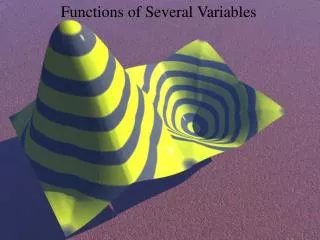
When we zoom in on a “sufficiently nice” function of two variables, we see a plane.
(a,b) Describing the Tangent Plane • To describe a tangent line we need a single number---the slope. • What information do we need to describe this plane? • Besides the point (a,b), we need two numbers: the partials of f in the x- and y-directions. Equation?
Describing the Tangent Plane We can also write this equation in vector form. Write x = (x,y), p = (a,b), and Gradient Vector! Dot product!
General Linear Approximations In the expression we can think of As a scalar function on 2: . This function is linear. Why don’t we just subsume F(p) into Lp? Linear--- in the linear algebraic sense.
General Linear Approximations In the expression we can think of As a scalar function on 2: . This function is linear. Note that the expression Lp(x-p) is not a product. It is the function Lpacting on the vector(x-p).
To understand Differentiability inVector Fields We must understand Linear Vector Fields: Linear Transformations from
Linear Functions A function L is said to be linear provided that Note that L(0) = 0, since L(x) = L (x+0) = L(x)+L(0). For a function L: m → n, these requirements are very prescriptive.
Linear Functions It is not very difficult to show that if L: m →nis linear, then L is of the form: where the aij’s are real numbers for j = 1, 2, . . . m and i =1, 2, . . ., n.
Linear Functions Or to write this another way. . . In other words, every linear function L acts just like left-multiplication by a matrix. Though they are different, we cheerfully confuse the function L with the matrix A that represents it! (We feel free to use the same notation to denote them both except where it is important to distinguish between the function and the matrix.)
One more idea . . . Suppose that A = (A1 , A2 , . . ., An) . Then for 1 j n Aj(x) = aj1 x1+aj 2 x2+. . . +aj n xn What is the partial of Aj with respect to xi?
One more idea . . . Suppose that A = (A1 , A2 , . . ., An) . Then for 1 j n Aj(x) = aj1 x1+aj 2 x2+. . . +aj n xn The partials of the Aj’s are the entries in the matrix that represents A!
Local Linear Approximation Suppose that F: m →nis given by coordinate functions F=(F1, F2, . . ., Fn) and all the partial derivatives of F exist at pin m and are continuous at pthen . . . there is a matrix Lp such that Fcan be approximated locally near p by the affine function What can we say about the relationship between the matrix DF(p)and the coordinate functions F1, F2, F3, . . ., Fn ? Quite a lot, actually. . . Lp will be denoted by DF(p) and will be called the Derivative of F at p or the Jacobian matrix of F at p.
A Deep Idea to take on Faith I ask you to believe that for all i and j with 1 i n and 1 j m This should not be too hard. Why? Think about tangent lines, think about tangent planes. Considering now the matrix formulation, what is the partial of Lj with respect to xi?
The Derivative of F at p(sometimes called the Jacobian Matrix of F at p) Notice the two common nomeclatures for the derivative of a vector –valued function.
In Summary. . . If F is a “reasonably well behaved” vector field around the point p, we can form the Jacobian Matrix DF(p). How should we think about this function E(x)? For all x, we have F(x)=DF(p) (x-p)+F(p)+E(x) where E(x) is the error committed by DF(p) +F(p) in approximating F(x).
E(x) for One-Variable Functions E(x) measures the vertical distance between f (x) and Lp(x) But E(x)→0 is not enough, even for functions of one variable! What happens to E(x) as x approaches p?
Definition of the Derivative • A vector-valued function F=(F1, F2, . . ., Fn)is differentiable at pin m provided that • All partial derivatives of the component functions • F1, F2, . . ., Fn of F exist on an open set containing p, and • The error E(x) committed by DF(p)(x-p)+F(p)in approximating F(x) satisfies • (Book writes this as • .)