Functions of Several Variables

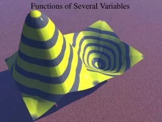
Functions of Several Variables Local Linear Approximation

Real Variables In our studies we have looked in depth at • functions f : X → Y where X and Y are arbitrary metric spaces, • real-valued functions f : X →  where X is an arbitrary metric space, and • functions f :  → . Now we want to look at functions f : n → m.

Scalar Fields A function F: n →  is called a Scalar Field because it assigns to each vector in n a scalar in . Scalar Fields: Think of the domain as a "field" in which each point is "tagged" with a number. Example: Each point in a room can be associated with a temperature in degrees Celsius.

Vector Fields A function F: n → m (m > 1) is called a Vector Field because it assigns to each vector in n a vector in m. Vector Fields: Think of the domain as a "field" in which each point is "tagged" with a vector. Example: domain is the surface of a river, we can associate each point with a current, which has both magnitude and direction and is therefore a vector.

Vector and Scalar Fields • Let F: n → m (m > 1) be a vector field. Then there are scalar fields F1, F2, . . . , Fm from n →  such that F(x) = (F1 (x), F2 (x), . . . , Fm (x) ) • The functions F1, F2, . . . , Fm are called the coordinate functions of F. • For example:

The Space n: Linear Algebra meets Analysis n is a Linear space (or vector space)---each element of n is a vector. Vectors can be added together and any vector multiplied by a scalar (number) is also a vector. n is Normed---Every element x in n has a norm ||x||, which is a non-negative real number and which you can think of as the “magnitude” of the vector.

x The Space n: Linear Algebra meets Analysis The norm of ||x|| is defined to be the (usual) distance in n from x to 0. The norm in  is analogous to the absolute value in :

Differentiability---1 variable • When we zoom in on a “sufficiently nice” function of one variable, we see a straight line.

Zooming and Differentiability • We expressed this view of differentiability by saying that f is differentiable at p if there exists a real number f’(p) such that provided that x is “close” to p. • More precisely, if for all x, In other words, if f is locally linear at p. where as x→p.

Functions of two Variables

When we zoom in on a “sufficiently nice” function of two variables, we see a plane.

(a,b) Describing the Tangent Plane • To describe a tangent line we need a single number---the slope. • What information do we need to describe this plane? • Besides the point (a,b), we need two numbers: the partials of f in the x- and y-directions. Equation?

Describing the Tangent Plane We can also write this equation in vector form. Write x = (x,y), p = (a,b), and Gradient Vector! Dot product!

General Linear Approximations In the expression we can think of the gradient as a linear function on 2. (It assigns a vector to each point in 2.) For a general function F: n → m and for a point p in n , we want to find a linear function Ap: n → m such that The function Ap is linear in the linear algebraic sense.

General Linear Approximations In the expression we can think of the gradient as a linear function on 2. (It assigns a vector to each point in 2.) For a general function F: n → m and for a point p in n , we want to find a linear function Ap: n → m such that Note that the expression Ap(x-p) is not a product. It is the function Apacting on the vector(x-p).

To understand Differentiability We need to understand Linear Functions

Linear Functions A function A is said to be linear provided that Note that A (0) = 0, since A(x) = A (x+0) = A(x)+A(0). For a function A: n →m, these requirements are very prescriptive.

Linear Functions It is not difficult to show that if A: n →mis linear, then A is of the form: where the aij’s are real numbers for i = 1, 2, . . . m and j =1, 2, . . ., n.

Linear Functions Or to write this another way. . . In other words, every linear function A acts just like left-multiplication by a matrix. Thus we cheerfully confuse the function A with the matrix that represents it!

Linear Algebra and Analysis The requirement that A: n →mbe linear is very prescriptive in other ways, too. • Let A be an mn matrix and the associated linear function. • Then A is Lipschitz with • In particular, when ||x||  1, • That is, A is bounded on the closed unit ball of n .

Norm of a Linear Function • We can thus define the norm of A: n →m by ||A|| = sup{ ||Ax|| : ||x||1}. • Properties of this norm: ||Ax||  ||A|| ||x|| for all x n . ||aA||=|a| ||A|| where a is a real number. ||BA||  ||B|| ||A|| (where B is an km matrix and A is an mn matrix.) BA represents the composition of B: m →k and A: n →m.

Norm of a Linear Function • Further properties of this norm: ||A+B||  ||A|| + ||B|| (where A and B are mn matrices.) ||aA||=|a| ||A|| where a is a real number. These two things imply that ||A-B|| is a distance function that measures the distances between linear functions from n to m. In other words, this norm on linear functions from n to m acts pretty much like the norm on n . To “first order” the properties that we associate with absolute values hold for this norm.

Local Linear Approximation For all x, we have F(x)=Ap(x-p)+F(p)+E(x) Where E(x) is the error committed by Lp(x)= Ap(x-p)+F(p) in approximating F(x)

Local Linear Approximation Fact: Suppose that F: n →mis given by coordinate functions F=(F1, F2, . . ., Fm) and all the partial derivatives of F exist “near” pn and are continuous at p, then . . . there is some matrix Ap such that Fcan be approximated locally near p by What can we say about the relationship between the matrix Ap and the coordinate functions F1, F2, F3, . . ., Fm ? Quite a lot, actually. . .

We Just Compute First, I ask you to believe that if Ap= (A1 , A2 , . . ., An)for all i and j with 1 i  n and 1  j m This should not be too hard. Why? Think about tangent lines, think about tangent planes. Considering now the matrix formulation, what is the partial of Aj with respect to xi? (Note: Aj(x) = aj 1 x1+aj 2 x2+. . . +ajn xn)

The Derivative of F at p(sometimes called the Jacobian Matrix of F at p)

Some Useful Derivatives • Identify the derivative of each vector field at a point p. Guess, then verify! • The constant function F (x) = v. • The identity function F(x) = x. • The Linear function A(x)=A x. • AF (Where A is a linear function and F is diff’able) • F+G (assuming both F and G are diff’able) • aF (where a and F is diff’able)

Continuity of the Derivative? Theorem: Suppose that all of the partial derivatives of F: n →m exist in a neighborhood around the point p and that they are all continuous at p. Then for every  > 0 there exists  > 0 such that if d (z , p) <  , then ||F’(z)- F’(p)|| < . In other words, if the partials exist and are continuous near p then the Jacobian matrix for p is “close” to the Jacobian matrix for any “nearby” point.

Mean Value Theorem for Vector Fields? Theorem: Let E be an open subset of n and let F: E → m. Suppose that a, b and the entire line segment joining them are in E. If F is differentiable at every point on the line segment between a and b (including the endpoints) then there exists c on the segment between a and b such that Note: does not hold if m >1! Even if n = 1 and m = 2.

Example? Standard way to interpret F: → 2 is to picture a (parametric) curve in the plane. Picture a fly flying around the curve. It’s velocity (a vector!) at any point is the derivative of the parametric curve at that point. What would mean for a closed curve?

The “Take Home Message” • The set of Linear Functions on n is normed and that norm behaves pretty much like the absolute value function. • There is a multi-variable version of the Mean Value Theorem than involves inequalities in the norms. • If the partials exist and are continuous, the Jacobian matrices corresponding to nearby points are “close” under the norm. I will remind you of these results when we need them.

Functions of Several Variables