Download
1 / 30
310 likes | 553 Vues
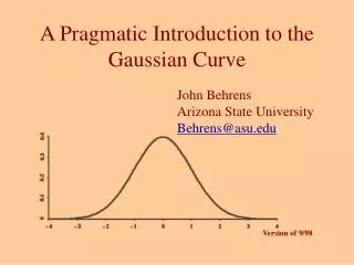
A Pragmatic Introduction to the Gaussian Curve. John Behrens Arizona State University Behrens @asu.edu. Version of 9/98. As we have seen, data occur in many shapes including. As we have seen, data occur in many shapes including. Positively Skewed.

E N D
A Pragmatic Introduction to the Gaussian Curve John Behrens Arizona State University Behrens@asu.edu Version of 9/98
As we have seen, data occur in many shapes including... • Positively Skewed
As we have seen, data occur in many shapes including... • Positively Skewed • Negatively Skewed WRITING
As we have seen, data occur in many shapes including... • Positively Skewed • Negatively Skewed • Bell-shaped
Curves with a single mode, and symmetric sides are often called . . . • Bell-shaped (remember the Liberty Bell?)
Curves with a single mode, and symmetric sides are often called . . . • Bell-shaped (remember the Liberty Bell?) • or Gaussian (after the mathematician who identified the exact shape)
Curves with a single mode, and symmetric sides are often called . . . • Bell-shaped (remember the Liberty Bell?) • or Gaussian (after the mathematician who identified the exact shape) • or “Normal” (a misnomer to get away from a dispute about authorship!).
Karl Pearson gave the name “Normal” to this shape: “Many years ago I called the Laplace-Gaussian curve the NORMAL curve, which name, while it avoids an international question of priority, has the disadvantage of leading people to believe that all other distributions of frequency are in one sense or another "abnormal." That belief is, of course, not justifiable.” Karl Pearson, 1920, p 25
Karl regretted it, and we will honor him by using the other terms. • Normalcy is a social, not a statistical concept. • In our culture, abnormal is valued in intelligence, but not in “moral” behavior. • Remember Adolph Quetelet and La Homme Moyen.
The Gaussian shape is not a general appearance, but a very specific shape. With a very specific formula:
0.4 0.3 0.2 0.1 0 What makes the shape Gaussian, is the relative height of the curve at the different locations • Whether the curve is tall -4 -3 -2 -1 0 1 2 3 4
0.4 0.3 0.2 0.1 0 What makes the shape Gaussian, is the relative height of the curve at the different locations • Whether the curve is tall • Or flat 0.4 0.3 0.2 0.1 0 -4 -3 -2 -1 0 1 2 3 4 -4 -3 -2 -1 0 1 2 3 4
0.4 0.3 0.2 0.1 0 What makes the shape Gaussian, is the relative height of the curve at the different locations • Whether the curve is tall • Or flat 0.4 0.3 0.2 0.1 0 -4 -3 -2 -1 0 1 2 3 4 • Each of these shapes are Gaussian, because of the relative height at each point of the horizontal scale. -4 -3 -2 -1 0 1 2 3 4
We have already talked about the peak of the distribution, which occurs at the mean.
Each side of the curve has inflection points where the curve makes shifts in direction.
Each side of the curve has inflection points where the curve makes shifts in direction.
1 SD The first inflection point to the right of the mean occurs one standard deviation above the mean. Mean Mean + 1 SD
Mean Mean + 1 SD + 2 SD The second inflection point to the right of the mean occurs two standard deviations above the mean. Mean
Mean Mean + 1 SD + 2 SD Inflection points below the mean occur at one and two standard deviations below the mean. Mean Mean Mean - 1 SD - 2 SD
Mean +1 SD +2 SD -1 SD -2 SD Because all points are in reference to the mean, we will indicate the differences with the mean implied.
Mean +1 SD +2 SD -1 SD -2 SD One of the most helpful aspects of the normal curve is that there are specific areas under each part of the curve.
50% 50% Mean +1 SD +2 SD -1 SD -2 SD As we noted before, 50% of the data falls on each side of the mean.
50% 50% 34% 34% Mean +1 SD +2 SD -1 SD -2 SD Of this 50%, 34% falls between the mean and one standard deviation above and below the mean.
50% 50% 34% 34% 14% 14% Mean +1 SD +2 SD -1 SD -2 SD The area between one and two standard deviations from the mean holds 14% of the distribution.
50% 50% 34% 34% 14% 14% Mean +1 SD +2 SD -1 SD -2 SD Since the total area on each side must sum to 50%, we know there is 2% of the distribution beyond two standard deviations in each direction. 2% 2%
Turn your attention to the tails for a moment. There are two things to notice. +2 SD +5 SD +3 SD +4 SD +6 SD
First, while most of the data is in the first few standard deviations, the tails go on forever. +2 SD +5 SD +3 SD +4 SD +6 SD
Second, notice that the 2% in the tails covers all the tails including the area of all subsequent standard deviations. When we work with all these areas, we will look their areas up in a table. +2 SD +5 SD +3 SD +4 SD +6 SD