Challenges in Data-Driven MHD Modeling of Magnetic Fields in the Solar Corona
230 likes | 350 Vues
This presentation discusses the integration of magnetic field observations into MHD models of the solar corona, highlighting the challenges associated with data-driven modeling. Key issues include determining electric fields consistent with photospheric magnetic field evolution, generating initial atmospheres based on X-ray observations, and incorporating new flux from separate systems into magnetized atmospheres. Advanced techniques like Minimum Energy Fitting (MEF) and Inductive Local Correlation Tracking (ILCT) are proposed for improving the accuracy of simulations, ultimately aiming for a more physically consistent representation of solar dynamics.

Challenges in Data-Driven MHD Modeling of Magnetic Fields in the Solar Corona
E N D
Presentation Transcript
Data-Driven Simulations of AR8210 W.P. Abbett Space Sciences Laboratory, UC Berkeley SHINE Workshop 2004
Incorporating Observations of Magnetic Fields into MHD Models of the Corona --- the Challenges: • Determining electric fields and flows consistent with the observed evolution of the magnetic field at the photosphere (Data-driven modeling) • Generating initial atmospheres consistent with X-ray observations of the corona (Relevant to both data-driven and “data-inspired” modeling) • Developing a physically-consistent means of incorporating newly emerging flux from a separate system into fully magnetized atmospheres (Critical to both data-driven and coupled models) • Developing standard techniques of testing and validating the new methods
Data-driven Modeling: Magnetic Fields and Flows at the Photosphere • MHD models require boundary flows (e.g., to update electric fields along the edges of control volumes within the boundary layers) that are consistent with the observed evolution of the magnetic field in the photosphere: • Note that the above system of equations is under-determined. • In the absence of simultaneous chromospheric and photospheric vector magnetograms, we cannot use data to directly update the transverse components of the magnetic field, since there is no means to specify the needed vertical gradients.
New Inversion Techniques • MEF (“Minimum Energy Fitting”): • Constrains the under-determined system by requiring that the spatially integrated square of the velocity field at the photosphere be minimized (Longcope & Regnier ApJ, 2004 in press) • ILCT: “Inductive Local Correlation Tracking”: • Uses velocities determined via local correlation tracking (applied to magnetic elements) along with the Demoulin & Berger (2003) hypothesis to generate all three components of a flow field that is consistent with both the observed evolution of the magnetic field and the vertical component of the ideal induction equation (Welsch, Fisher, Abbett & Regnier, ApJ 2004 in press) • “Minimum Structure Reconstruction”: Poster #51 SHINE 2004 (Georgoulis, M., & LeBonte, B. J.)
ILCT Consider the ideal induction equation: ∂B/∂t = x (v x B) Re-cast the z-component of the induction equation as: ∂Bz/∂t + · (vBz − vzB) = 0 Define a new quantity U as: U v − (B/Bz)vz (equivalent to the Demoulin & Berger 2003 hypothesis) Then we have ∂Bz/∂t + · (BzU) = 0
Note that only flows perpendicular to the magnetic field affect the evolution of B, thus we have the freedom to set v·B=0 Then if we can somehow determine U, we can obtain v and vz via a simple algebraic decomposition: vz = (U·B)Bz/B 2 v = U − (U·B) B/B 2 But LCT techniques applied to magnetic elements return a quantity “u(LCT)” that in practice differs from the true U . ILCT
ILCT • Then let’s define scalar quantities φ and ψ in the following way: Bzu −φ + x (ψz) • Taking the curl of both sides of the equation gives a Poisson equation for ψ: x (Bzu) = −2 ψ • If we now assume that ucan be approximated by u(LCT) in the above equation we can determine ψ. If we now require that ualso satisfy the induction equation, we can write: Bzu= vBz − vzB = −φ + x (ψz) • and the induction equation thus constrains φ: ∂Bz/∂t = −2 φ
ILCT • Then all that remains is to solve two Poisson equations to obtain φ and ψ (problem solved!) • Note that only the vertical component of the magnetic field is required to find a solution consistent with the z-component of the induction equation! • Given the transverse magnetic field from a vector magnetogram, we can obtain a physically self-consistent flow field suitable for incorporation into the lower boundary of MHD models of the corona.
Testing Inversion Techniques (see Welsch et al. poster #50) • Apply the inversion techniques to magnetic fields and flows obtained from simulations of surface and sub-surface active-region magnetic fields • Radiative MHD simulations of the surface layers can also provide a test of LCT techniques applied to intensity features
Generating an Initial State: • We need more than just a physically consistent scheme to update the photospheric boundary --- we also need an initial specification of all components of the magnetic field throughout the domain that compares favorably with e.g. soft X-ray images of the corona (see poster #49 Barnes et al. for a discussion of “compares favorably”). • Challenges: • The magnetic configuration of a complex active region is highly non-potential • The atmosphere below the chromosphere is not force-free • Best solution (at the moment!): Perform a non-linear force-free extrapolation • Note however, not all techniques produce results that can be used to initiate MHD models (e.g. mismatches in the transverse field at the lower boundary are problematic)
Generating an Initial State: Testing Extrapolation Techniques Against MHD Simulations of Flux Emergence Synthetic “magnetograms” taken at different heights in the model atmosphere from the model photosphere to the model chromosphere (bottom right). from Magara et al. 2004. • A comparison of a local PFSS and the Wheatland et al. 2000 non-constant-alpha force-free extrapolation technique applied to the Magara 2004 MHD simulation of flux emergence (from Abbett et al. 2004)
Generating an Initial State: AR-8210 • Above: Wheatland et al. 2000 method applied to NOAA AR-8210 (May 1, 1998) --- from J. M. McTiernan • Note that to compare with observed X-ray emission, one must perform additional calculations: e.g., assume a loop heating mechanism and solve the energy equation along individual loops (Lundquist, Schrijver)
Emerging Flux into a Fully Magnetized Model Corona • Calculations like the one shown on the left represent a very simple case: here, sub-photospheric flux emerges into an initially field-free model atmosphere • If we now assume that the model corona is initially filled with field, we must consider how the pre-existing structure interacts with the introduction of new flux when updating the boundary values. A simulation of flux emergence into an initially field-free model corona (from Abbett & Fisher 2003). The color table indicates the degree to which the model corona is force-free during the dynamic emergence process.
Emerging Flux into a Fully Magnetized Model Corona • To address this problem, an assumption must be made: in our case, we choose to ignore the back-reaction from coronal forces --- that is, we assume that photospheric flows dominate the dynamics of the boundary layer. • Then the ideal induction equation is linear, and we can express the magnetic field in the boundary layer as a superposition of two vector fields B = B1+ B2: ∂(B1+B2)/∂t = x v1 x (B1 + B2) • Here, v1 represents the imposed boundary flow; B1 represents new flux introduced into the system from below (assumed zero at t=0); and B2, which at t=0 represents the portion of the initial coronal flux system that permeates the boundary layers. • Since the emerging flux system satisfies ∂B1/∂t= x (v1 x B1), B2(t=0) is known, and v1 is specified for all t, we can advance B2 in time, and thus specify a boundary field B that satisfies the ideal MHD induction equation for all time t, given a standard boundary condition for B2.
Emerging Flux into a Fully Magnetized Model Corona • Of course, this treatment allows for differences between the magnetic field imposed in the boundary layers and the vector field observed at the photosphere. • If we impose a further condition, and require that the vertical component of the field evolve exactly in accordance with the z-component of the field observed at the photosphere, our previous condition can be re-cast as: ∂B/∂t = x v1 x B1 + x z [(v1 x B2)·z] ˆ ˆ • In this approximation, we neglect the components of ∂B2/∂t= x (v1 x B2) that either alter the prescribed evolution of Bz at the boundary, z· (∂B2/∂t), or involve vertical gradients of B2.
Emerging Flux into a Fully Magnetized Model Corona • We demonstrate the previous technique by driving the SAIC model corona with the vector magnetic field obtained from an ANMHD sub-surface simulation. • We emerge flux into a pre-existing dipole field: In one case, the arcade field has an opposite polarity to that of the emerging bipole, and in another case the arcade field has the same polarity. • Consider this a “test run” for a data-driven calculation Image from Abbett, Mikic, Linker et al. 2004
Putting it all Together • Two fully-coupled codes: • Boundary code: Flows prescribed by ILCT; the magnetic induction equation, continuity equation and a simple energy equation are solved implicitly in a thin boundary layer • MHD corona: the system of ideal MHD equations are solved on a non-uniform grid; the boundary code is fully coupled to the model corona.
Simulation of AR-8210: The Boundary Layers • Vertical magnetic field from a 3D calculation initiated by an IVM vector magnetogram of AR-8210 at 19:40 (Regnier), and a NLFFF extrapolation (McTiernan) • The simulation is driven by ILCT flows applied to the magnetogram at 19:40, and one approximately four hours later
Progress: • Developed necessary inversion techniques • Developed 3D boundary code, and applied it to AR-8210 as a test of the inversion technique • Coupled boundary code to 3D MHD corona Remaining Challenges: • Incorporate global topology into the local model corona • Refine lower boundary condition (energetics, temporal scaling, flows parallel to the magnetic field)