Discriminative and Generative Recognition
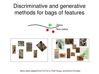
CS 636 Computer Vision. Discriminative and Generative Recognition. Nathan Jacobs. Slides adapted from Lazebnik. Discriminative and generative methods for bags of features. Zebra. Non-zebra. Many slides adapted from Fei-Fei Li, Rob Fergus, and Antonio Torralba. Image classification.

Discriminative and Generative Recognition
E N D
Presentation Transcript
CS 636 Computer Vision Discriminative and Generative Recognition Nathan Jacobs Slides adapted from Lazebnik
Discriminative and generative methods for bags of features Zebra Non-zebra Many slides adapted from Fei-Fei Li, Rob Fergus, and Antonio Torralba
Image classification • Given the bag-of-features representations of images from different classes, how do we learn a model for distinguishing them?
Discriminative methods • Learn a decision rule (classifier) assigning bag-of-features representations of images to different classes Decisionboundary Zebra Non-zebra
Classification • Assign input vector to one of two or more classes • Any decision rule divides input space into decision regions separated by decision boundaries
Nearest Neighbor Classifier • Assign label of nearest training data point to each test data point from Dudaet al. Voronoi partitioning of feature space for two-category 2D and 3D data Source: D. Lowe
K-Nearest Neighbors • For a new point, find the k closest points from training data • Labels of the k points “vote” to classify • Works well provided there is lots of data and the distance function is good k = 5 Source: D. Lowe
Functions for comparing histograms • L1 distance • χ2 distance • Quadratic distance (cross-bin) Jan Puzicha, Yossi Rubner, Carlo Tomasi, Joachim M. Buhmann: Empirical Evaluation of Dissimilarity Measures for Color and Texture. ICCV 1999
Earth Mover’s Distance • Each image is represented by a signatureS consisting of a set of centers {mi } and weights {wi} • Centers can be codewords from universal vocabulary, clusters of features in the image, or individual features (in which case quantization is not required) • Earth Mover’s Distance has the formwhere the flowsfij are given by the solution of a transportation problem Y. Rubner, C. Tomasi, and L. Guibas: A Metric for Distributions with Applications to Image Databases. ICCV 1998
Moving Earth ≠ Slides by P. Barnum
The Difference? (amount moved) =
The Difference? (amount moved) * (distance moved) =
Earth Mover’s Distance Can be formulated as a linear program… a transportation problem. =
Y. Rubner, C. Tomasi, and L. J. Guibas. A Metric for Distributions with Applications to Image Databases. ICCV 1998
Why might EMD be better or worse than these? • L1 distance • χ2 distance • Quadratic distance (cross-bin) Jan Puzicha, Yossi Rubner, Carlo Tomasi, Joachim M. Buhmann: Empirical Evaluation of Dissimilarity Measures for Color and Texture. ICCV 1999
recall: K-Nearest Neighbors • For a new point, find the k closest points from training data • Labels of the k points “vote” to classify • Works well provided there is lots of data and the distance function is good k = 5 Source: D. Lowe
Linear classifiers • Find linear function (hyperplane) to separate positive and negative examples Why not just use KNN? Which hyperplane is best?
Support vector machines • Find hyperplane that maximizes the margin between the positive and negative examples C. Burges, A Tutorial on Support Vector Machines for Pattern Recognition, Data Mining and Knowledge Discovery, 1998
Support vector machines • Find hyperplane that maximizes the margin between the positive and negative examples For support vectors, Distance between point and hyperplane: Therefore, the margin is 2 / ||w|| Support vectors Margin C. Burges, A Tutorial on Support Vector Machines for Pattern Recognition, Data Mining and Knowledge Discovery, 1998
What if they aren’t separable? Quadratic optimization problem: Subject to yi(w·xi+b) ≥ 1 separable formulation Quadratic optimization problem: Subject to yi(w·xi+b) ≥ 1 – si si≥ 0 non-separable formulation
Introducing the “Kernel Trick” • Notice: learned weights support vector C. Burges, A Tutorial on Support Vector Machines for Pattern Recognition, Data Mining and Knowledge Discovery, 1998
Introducing the “Kernel Trick” • Recall:w·xi + b= yifor any support vector • Classification function (decision boundary): • Notice that it relies on an inner product between the testpoint xand the support vectors xi • Solving the optimization problem can also be done with only the inner products xi· xjbetween all pairs oftraining points C. Burges, A Tutorial on Support Vector Machines for Pattern Recognition, Data Mining and Knowledge Discovery, 1998
x 0 x 0 x2 Nonlinear SVMs • Datasets that are linearly separable work out great: • But what if the dataset is just too hard? • We can map it to a higher-dimensional space: 0 x Slide credit: Andrew Moore
Nonlinear SVMs • General idea: the original input space can always be mapped to some higher-dimensional feature space where the training set is separable: Φ: x→φ(x) Lifting Transformation Slide credit: Andrew Moore
Nonlinear SVMs • The kernel trick: instead of explicitly computing the lifting transformation φ(x), define a kernel function K such thatK(xi,xj) = φ(xi)· φ(xj) • This gives a nonlinear decision boundary in the original feature space: C. Burges, A Tutorial on Support Vector Machines for Pattern Recognition, Data Mining and Knowledge Discovery, 1998
Kernels for bags of features • Histogram intersection kernel: • Generalized Gaussian kernel: • D can be Euclidean distance, χ2 distance, Earth Mover’s Distance, etc. J. Zhang, M. Marszalek, S. Lazebnik, and C. Schmid, Local Features and Kernels for Classifcation of Texture and Object Categories: A Comprehensive Study, IJCV 2007
Summary: SVMs for image classification • Pick an image representation (in our case, bag of features) • Pick a kernel function for that representation • Compute the matrix of kernel values between every pair of training examples • Feed the kernel matrix into your favorite SVM solver to obtain support vectors and weights • At test time: compute kernel values for your test example and each support vector, and combine them with the learned weights to get the value of the decision function
What about multi-class SVMs? • Unfortunately, there is no “definitive” multi-class SVM formulation • In practice, we have to obtain a multi-class SVM by combining multiple two-class SVMs • One vs. others • Traning: learn an SVM for each class vs. the others • Testing: apply each SVM to test example and assign to it the class of the SVM that returns the highest decision value • One vs. one • Training: learn an SVM for each pair of classes • Testing: each learned SVM “votes” for a class to assign to the test example
SVMs: Pros and cons • Pros • Many publicly available SVM packages:http://www.kernel-machines.org/software • Kernel-based framework is very powerful, flexible • SVMs work very well in practice, even with very small training sample sizes • Cons • No “direct” multi-class SVM, must combine two-class SVMs • Computation, memory • During training time, must compute matrix of kernel values for every pair of examples • Learning can take a very long time for large-scale problems
Summary: Discriminative methods • Nearest-neighbor and k-nearest-neighbor classifiers • L1 distance, χ2 distance, quadratic distance, Earth Mover’s Distance • Support vector machines • Linear classifiers • Margin maximization • The kernel trick • Kernel functions: histogram intersection, generalized Gaussian, pyramid match • Multi-class • Of course, there are many other classifiers out there • Neural networks, boosting, decision trees, …
likelihood prior posterior Generative learning methods for bags of features • Model the probability of a bag of features given a class Many slides adapted from Fei-Fei Li, Rob Fergus, and Antonio Torralba
Generative methods • We will cover two models, both inspired by text document analysis: • Naïve Bayes • Probabilistic Latent Semantic Analysis
The Naïve Bayes model • Start with the likelihood Csurka et al. 2004
The Naïve Bayes model • Assume that each feature is conditionally independent given the class fi: ith feature in the image N: number of features in the image Csurka et al. 2004
The Naïve Bayes model • Assume that each feature is conditionally independent given the class fi: ith feature in the image N: number of features in the image wj: jth visual word in the vocabulary M: size of visual vocabulary n(wj): number of features of type wj in the image Csurka et al. 2004
The Naïve Bayes model • Assume that each feature is conditionally independent given the class No. of features of type wj in training images of class c Total no. of features in training images of class c p(wj| c) = Csurka et al. 2004
The Naïve Bayes model • Assume that each feature is conditionally independent given the class No. of features of type wj in training images of class c + 1 Total no. of features in training images of class c + M p(wj| c) = (psuedocounts to avoid zero counts) Csurka et al. 2004
The Naïve Bayes model • Maximum A Posteriori decision: (you should compute the log of the likelihood instead of the likelihood itself in order to avoid underflow) Csurka et al. 2004
The Naïve Bayes model • “Graphical model”: c w N Csurka et al. 2004
Probabilistic Latent Semantic Analysis = p1 + p2 + p3 Image zebra grass tree “visual topics” T. Hofmann, Probabilistic Latent Semantic Analysis, UAI 1999
z d w Probabilistic Latent Semantic Analysis • Unsupervised technique • Two-level generative model: a document is a mixture of topics, and each topic has its own characteristic word distribution document topic word P(z|d) P(w|z) T. Hofmann, Probabilistic Latent Semantic Analysis, UAI 1999
z d w Probabilistic Latent Semantic Analysis • Unsupervised technique • Two-level generative model: a document is a mixture of topics, and each topic has its own characteristic word distribution T. Hofmann, Probabilistic Latent Semantic Analysis, UAI 1999
The pLSA model Probability of word i giventopic k (unknown) Probability of word iin document j(known) Probability oftopic k givendocument j(unknown)
The pLSA model documents topics documents p(wi|dj) p(wi|zk) p(zk|dj) words words topics = Class distributions per image (K×N) Observed codeword distributions (M×N) Codeword distributions per topic (class) (M×K)
Learning pLSA parameters Maximize likelihood of data: Observed counts of word i in document j M … number of codewords N … number of images Slide credit: Josef Sivic
Inference • Finding the most likely topic (class) for an image:
Inference • Finding the most likely topic (class) for an image: • Finding the most likely topic (class) for a visual word in a given image:
Topic discovery in images J. Sivic, B. Russell, A. Efros, A. Zisserman, B. Freeman, Discovering Objects and their Location in Images, ICCV 2005